Syntax:
surf_collide ID style args keyword values ...
  specular or specular/kk args = noslip (optional)
    noslip = reflect all velocity components off surface (not just normal component)
  diffuse or diffuse/kk args = Tsurf acc
    Tsurf = temperature of surface (temperature units)
            Tsurf can be a variable or custom per-surf attribute (see below)
    acc = accommodation coefficient
  cll args = Tsurf acc_n acc_t acc_rot acc_vib
    Tsurf = temperature of surface (temperature units)
            Tsurf can be a variable or custom per-surf attribute (see below)
    acc_n = accommodation coefficient in the surface normal direction
    acc_t = accommodation coefficient in the surface tangential direction
    acc_rot = accommodation coefficient for the rotational modes
    acc_vib = accommodation coefficient for the vibrational modes
  adiabatic args = none
  impulsive args = Tsurf model param1 param2 var theta_peak pol_pow azi_pow
    Tsurf = temperature of surface (temperature units)
            Tsurf can be a variable or custom per-surf attribute (see below)
    model can be softsphere or tempvar
      softsphere args = en_ratio eff_mass
        param1 = en_ratio = fraction of energy lost in the collision
        param2 = eff_mass = effective mass of the surface atom
      tempvar args = a1 a0
        param1 = a1 = linear term in the variation with temperature
        param2 = a0 = constant term in the variation with temperature
    var = variance of the scattered particle velocity distribution
    theta_peak = peak location of the polar angle distribution
    pol_pow = cosine power represeting the polar angular distribution
    azi_pow = cosine power represeting the azimuthal angular distribution
  td arg = Tsurf
    Tsurf = temperature of surface (temperature units)
            Tsurf can be a variable or custom per-surf attribute (see below)
  piston or piston/kk args = Vwall
    Vwall = velocity of boundary wall (velocity units)
  transparent or transparent/kk args = none
vanish or vanish/kk args = none
  translate args = Vx Vy Vz
    Vx,Vy,Vz = translational velocity of surface (velocity units)
  rotate args = Pz Py Pz Wx Wy Wz
    Px,Py,Pz = point to rotate surface around (distance units)
    Wx,Wy,Wz = angular velocity of surface around point (radians/time)
  temp/freq arg = Nfreq
    Nfreq = evaulate a temperature variable every this many timesteps (default = 1)
  partial args = eccen (only for cll style)
    eccen = eccentricity parameter
  barrier args = bar_val (only for td style)
    bar_val = value of the desorption barrier in temperature units
  bond args = bond_trans bond_rot bond_vib (only for td style)
    bond_trans = amount of bond dissociation energy (in temperature units) going into translational mode
    bond_rot = amount of bond dissociation energy (in temperature units) going into rotational mode
    bond_vib = amount of bond dissociation energy (in temperature units) going into vibrational mode
  init_energy = IE_trans IE_rot IE_vib (only for td style)
    IE_trans = fraction of initial translational energy going into translational mode
    IE_rot = fraction of initial translational energy going into rotational mode
    IE_vib = fraction of initial translational energy going into vibrational mode
  step args = epsilon (only for impulsive style)
    epsilon = ratio of the height to the width of the step
  double args = polar_pow_2 (only for impulsive style)
    polar_pow_2 = cosine power for the polar angular distribution between peak and surface
  intenergy args = frac_rot frac_vib (only for impulsive style)
    frac_rot = fraction of lost translational energy going into the rotational mode
    frac_vib = fraction of lost translational energy going into the vibrational mode
Examples:
surf_collide 1 specular
surf_collide 1 transparent
surf_collide 1 diffuse 273.15 0.9
surf_collide 1 cll 273.15 0.8 0.8 0.5 0.1
surf_collide 1 cll 273.15 1.0 1.0 0.1 0.1 partial 0.5
surf_collide 1 adiabatic
surf_collide 1 impulsive 1000.0 softsphere 0.2 50 2000 60 5 75
surf_collide 1 impulsive 1000.0 tempvar 3 500 2000 60 5 75
surf_collide 1 impulsive 1000.0 softsphere 0.2 50 2000 60 5 75 double 10
surf_collide 1 impulsive 1000.0 tempvar 3 500 2000 60 5 75 step 0.1
surf_collide heatwall diffuse v_ramp 0.8 temp/freq 100
surf_collide heatwall diffuse v_ramp 0.8 translate 5.0 0.0 0.0
Description:
Define a model for particle-surface collisions. One or more models can be defined and assigned to different surfaces or simulation box boundaries via the surf_modify or bound_modify commands. See >Section 4.9 for more details of how SPARTA defines surfaces as collections of geometric elements, triangles in 3d and line segments in 2d. Chemical reactions can also be part of a particle-surface interaction model. See the surf_react command for details. All of the collision styles listed here support optional reactions, except the vanish style.
The ID for a surface collision model is used to identify it in other commands. Each surface collision model ID must be unique. The ID can only contain alphanumeric characters and underscores.
Several of the surface collision models specify Tsurf as an argument for the temperature of the surface. It can be specified in three different ways.
First, Tsurf can be a numeric value. The temperature of all surface elements assigned to the model will be the same and will be constant for the duration of the simulation.
Second, Tsurf can be a variable specified as v_name where name is the name of the variable defined by the variable command. Two different styles of variable can be used.
The first is an equal-style variable which evaulates to a single scalar value, which will be the temperature assigned to every surface element. Equal-style variables can specify formulas with various mathematical functions, and include stats_style command keywords and timestep and elapsed time. Thus it is easy to specify a time-dependent temperature.
The second is a surf-style variable with a formula which can calculate a different temperature for each surface element, e.g. a temperature which depends on the geometric location of the center point of the surface element. The calculation can also be time-dependent if desired. A surf-style variable can also access a compute or fix which outputs per-surf quantities. For example the compute surf and fix ave/surf commands can tally or average energy transfer from particles to surface elements, which could be used to infer a temperature for each surface element.
Note that the frequency at which the equal-style or surf-style variable is evaluated can be set using the optional temp/freq keyword, disussed below. The default value is 1, meaning the variable is evaluated every timestep. Surf-style variables can be expensive to evaluate, because they require inter-processor communication in parallel, so you may wish to set the temp/freq keyword to a larger value.
Third, Tsurf can be a custom per-surf attribute specified as s_name with the name of the attribute. It must be a custom per-surf vector with floating point values for the temperature for each surface element. These could be static values initialized, for example, by the read_surf command. Or they could be dynamic values recomputed periodically, for example, by the "fix surf/temp" command. See Section 6.17 for more discussion of custom attributes.
Note that if the custom per-surf vector values are dynamic, then each time they are modified (e.g. by the fix surf/temp command), then their use by a surf_collide model will trigger inter-processor communication to ensure each processor knows the correct temperature values for the surface elements its particles interact with. This can be an expensive operation, so it may be desirable to not update the custom per-surf vector values too frequently.
The specular style computes a simple specular reflection model. It requires no arguments. Specular reflection means that a particle reflects off a surface element with its incident velocity vector reversed with respect to the outward normal of the surface element. The particle's speed is unchanged.
Specular reflection means that a particle bounce off a surface element reverses only the component of its velocity normal to the surface. If the optional noslip keyword is used, the particle bounce flips the sign of all 3 xyz components of the particle's incident velocity, so that it now moves in the opposite direction, creating a no slip boundary condition. In either case, the particle's speed is unchanged.
The diffuse style computes a simple diffusive reflection model.
The model has 2 parameters set by the Tsurf and acc arguments.
The Tsurf argument specifies the temperature of the surface. It can be a numeric value, surf-style variable, or custom per-surf attribute. See the explanation for all 3 options above.
Acc is an accommodation coefficient from 0.0 to 1.0, which determines what fraction of surface collisions are diffusive. The rest are specular. Thus a setting of acc = 0.0 means all collisions are specular.
Note that setting acc = 0.0, is a way to perform surface reactions with specular reflection, via the surf_react command, which cannot be done in conjunction with the surf_collide specular command. See the surf_react doc page for details.
Diffuse reflection emits the particle from the surface with no dependence on its incident velocity. A new velocity is assigned to the particle, sampled from a Gaussian distribution consistent with the surface temperature. The new velocity will have thermal components in the direction of the outward surface normal and the plane tangent to the surface given by:
The cll style computes the surface collision model proposed by Cercignani, Lampis and Lord. The model has 5 parameters set by the Tsurf, acc_n, acc_t, acc_rot, and acc_vib arguments.
The Tsurf argument specifies the temperature of the surface. It can be a numeric value, surf-style variable, or custom per-surf attribute. See the explanation for all 3 options above.
Acc_n, acc_t, acc_rot, and acc_vib are the accommodation coefficient for the surface normal direction, surface tangential directions, rotational energy mode, and vibrational energy mode respectively. The rotational and vibrational energy accommodation values must be specified even for an atomic species; however these values are simply ignored.
The theoretical scattering kernel was proposed by Cercignani and Lampis (Cercignani71). In this original model, two accommodation coefficients for the normal and tangential directions are employed. Each of these quantities can take a value between 0 and 1. Specular reflection is achieved by using the values (0,0), while complete thermal accommodation with the surface and cosine angular distributions is obtained using (1,1). There is smooth variation of both the energy and angular distribution for values in between these limits leading to lobular distributions similar to those observed in experiments. The implementation details of this model within DSMC was given by Lord (Lord90), along with extension to rotational and vibrational modes with both continuous and discrete levels (Lord91).
The adiabatic style computes the adiabatic surface collision model proposed by Mohammadzadeh, Rana, and Struchtrup (Mohammadzadeh16). This style requires no arguments. The adiabatic surface is modelled by scattering particles isotropically whilst conserving their velocity magnitude. Therefore, no energy is transferred between the wall and the particles. Note, that this is only valid for particle collisions not for potential surface reactions.
The td style computes the thermal desorption surface collision model proposed by Swaminathan Gopalan et al. (SG18), which is similar to diffuse style with an accommodation coefficient acc = 1.0.
The Tsurf argument specifies the temperature of the surface. It can be a numeric value, surf-style variable, or custom per-surf attribute. See the explanation for all 3 options above.
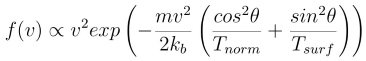
The particles are scattered thermally based on the Maxwell Boltzmann distribution conisstent with the surface temperture. The new velocity will have thermal components in the direction of the outward surface normal and the plane tangent to the surface given by:
The impuslive style computes the surface collision model proposed by Swaminathan Gopalan et al. (SG18). The model has 8 parameters. Within impulsive scattering, two different models are available, namely softsphere and tempvar. The softsphere argument uses the soft sphere model and has two parameters: en_ratio which represents the fraction of energy lost during the collision, and eff_mass specifying the effective mass of the surface atom. The tempvar argument directly provides the peak value of the scattered particle velocity distribution as a linear function of temperature. It has two parameters: the linear term a1 and constant term a0. The other five parameters Tsurf, var, pol_peak, pol_pow, azi_pow are set for both the models.
The Tsurf argument specifies the temperature of the surface. It can be a numeric value, surf-style variable, or custom per-surf attribute. See the explanation for all 3 options above.
Var is the variance of the scattered particle velocity distribution; pol_peak is the peak of the polar angle distribution; pol_pow and azi_pow are the cosine power representing the polar and azimuthal angle distribution respectively.
The impulsive model is used to represent the scattering of particles having super or hyperthermal translational energies and very low internal energies, like in a beam. This type of scattering falls under the structural regime, whose scattering physics and distributions are very different from the thermal regime. The velocity distribution of the impulsive scattering model can be represented using a Gaussian distribution with a mean u0 and a variance \alpha following Rettner (Rettner94a)
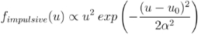
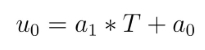
The variance parameter is directly specified by the user. The value of u0 can be provided directly using the tempvar model in which it is represented as a linear function of temperature. The linear term a1 and constant term a0 are given as inputs.

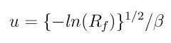
The u0 parameter can also be specified by a more physical model such as the soft sphere scattering model (Alexander12). This model uses the parameters en_ratio, the fraction of energy lost in the collision and eff_mass, the effective mass of the surface atom to determine the average final energy and then the average final velocity u0. Within the soft sphere model, the average final velocity will vary as a function of the final polar angle.
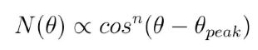
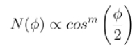
Both the polar and azimuthal angular distribution are lobular in nature and sharply peaked. These distributions can be represented using the cosine power law distribution Glatzer97. The peak of the azimuthal distribution remains at zero, while the peak of the polar angle distribution is usually higher than the incident angle (away from the normal). Hence the peak location (\theta_peak) and cosine power (n) of the polar angle distribution and the cosine power (m) of the azimuthal angular distribution are taken as input parameters. A factor of 2 is present in the azimuthal distribution to ensure the function remians positive within the range of the azimuthal angle: (-180, 180)
The internal (rotational and vibrational) energy of an incident molecule remains unchanged within the impulsive model unless the optional keyword intenergy is specified (see below).
The piston style models a subsonic pressure boundary condition. It can only be assigned to the simulation box boundaries via the bound_modify command or to surface elements which are parallel to one of the box boundaries (via the surf_modify command).
It treats collisions of particles with the surface as if the surface were moving with specified velocity Vwall away from the incident particle. Thus the "collision" actually occurs later in the timestep and the reflected velocity is less than it would be for reflection from a stationary surface. This calculation is performed using equations 12.30 and 12.31 in (Bird94)) to compute the reflected velocity and final position of the particle. If the particle does not return within the timestep to a position inside the simulation box (for a boundary surface) or to the same side of the initial surface that it started from (for a surface element collision), the particle is deleted. This effectively induces particles at the boundary to have a velocity distribution consistent with a subsonic pressure boundary condition, as explained in (Bird94)).
Vwall should be chosen to correspond to a desired pressure condition for the density of particles in the system.
NOTE: give more details on how to do this?
Note that Vwall must always be input as a value >= 0.0, meaning the surface is moving away from the incident particle. For example, in the z-dimension, if the upper box face is assigned Vwall, it is moving upward. Similarly if the lower box face is assigned Vwall, it is moving downward.
The transparent style simply allows particles to pass through the surface without altering the particle properties.
This is useful for tallying flow statistics. The surface elements must have been flagged as transparent when they were read in, via the read_surf command and its transparent keyword. The compute surf command will tally fluxes differently for transparent surf elements. The Section 6.15 doc page provides an overview of transparent surfaces. See those doc pages for details.
The vanish style simply deletes any particle which hits the surface.
This is useful if a surface is defined to be an inflow boundary on the simulation domain, e.g. using the fix emit/surf command. Using this surface collision model will also treat the surface as an outflow boundary. This is similar to using the fix emit/face command on a simulation box face while also setting the face to be an outflow boundary via the boundary o command.
Note that the surf_react global command can also be used to delete particles hitting a surface, by setting the pdelete parameter to 1.0. Using a surf_collide vanish command is simpler.
The keyword translate can only be applied to the diffuse and cll style. It models the surface as if it were translating with a constant velocity, specified by the vector (Vx,Vy,Vz). This velocity is added to the final post-collisional velocity of each particle that collides with the surface.
The keyword rotate can only be applied to the diffuse and cll style. It models the surface as if it were rotating with a constant angular velocity, specified by the vector W = (Wx,Wy,Wz), around the specified point P = (Px,Py,Pz). Note that W and P define the rotation axis. The magnitude of W defines the speed of rotation. I.e. if the length of W = 2*pi then the surface is rotating at one revolution per time unit, where time units are defined by the units command.
When a particle collides with the surface at a point X = (x,y,z), the collision point has a velocity given by V = (Vx,Vy,Vz) = W cross (X-P). This velocity is added to the final post-collisional velocity of the particle.
The rotate keyword can be used to treat a simulation box boundary as a rotating wall, e.g. the end cap of an axisymmetric cylinder. Or to model a rotating object consisting of surface elements, e.g. a sphere. In either case, the wall or surface elements themselves do not change position due to rotation. They are simply modeled as having a tangential velocity, as if the entire object were rotating.
IMPORTANT NOTE: For both the translate and rotate keywords the added velocity can only be tangential to the surface, with no normal component since the surface is not actually moving in the normal direction. SPARTA does not check that the specified translation or rotation produces a tangential velocity. However if does enforce the condition by subtracting off any component of the added velocity that is normal to the simulation box boundary or individual surface element.
The temp/freq keyword only applies to the styles which define a Tsurf parameter for the temperature of the surface, and also only applies if Tsurf is specified as a variable with the syntax v_name. The Nfreq value determines the frequency at which the variable is evaluated, once every Nfreq timesteps. The default value is 1 (evaluate every timestep). This is usually fine for equal-style variables, but surf-style variables may be expensive to evaluate. In which case setting Nfreq to 100 or 1000 may be desirable.
The keyword partial can only be applied to the cll style. Within the CLL model, the energy and angular distribution are linked. Lord (Lord95) proposed a way to decouple the energy accommodation from the angular distribution. This case of partially diffuse scattering with incomplete energy accommodation can be activated in SPARTA using the optional keyword partial. It requires an additional parameter eccentricity set by the eccen argument. For this case, the energy accommodation is calculated using the accommodation coefficients, but the angular distribution is computed using the additional parameter eccentricity. The eccen parameter can vary between 0 and 1. A value of 0 represents fully diffuse scattering and gives a cosine angular distribution. Increasing value of eccen presents more peaked and lobular distribution (Lord95).
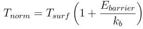
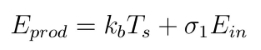
The keywords barrier, bond, and initenergy can only be applied to the td style. Due to the nature of the interaction between the products and the surface, the desorption of the products might have an energy barrier. For a surface desorption process, this desorption barrier exists only in the normal direction. Thus, only the products having enough energy (in the normal direction) to overcome the barrier will be able to desorb from the surface. This alters the velocity distribution of the observed products along the surface normal direction and thus leads to the distortion of the speed distribution (Goodman72). The angular distributions, which represent the ratio of the normal to the tangential velocities, are also altered as a result of the desorption barrier. The angular distributions are peaked more towards the normal and are often described by a cosine power law distribution.
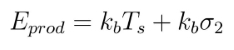
In addition to the desorption energy barrier, products formed through thermal mechanisms might have energies exceeding those corresponding to the bulk surface temperature. The energy of the local surface environment where the product formation occurs might be greater than the normal surface temperature due to the formation of local hot-spots (Rettner94b).
These hot-spots might stem from the dissociation or bond energy of the intermediates or the products. The optional keyword bond can be used to account for this scenario. This requires three arguments: the amount of energy (in temperature units) going into the translational, rotational and vibrational mode.
The higher energy during desorption might also arise due to the energy deposited by high speed of the incoming gas-phase particles. Since the formation of the products is rapid, the product might form and desorb before this high energy dissipates from the local hot-spots (Beckerle90). In this case, although the products are in thermal equilibrium with the surroundings, the energies of the products might not depend only on the equilibrium surface temperature, but also on the incoming velocities of the particles. This can be used within SPARTA using the optional keyword initenergy. It requires 3 arguments: fraction of the initial translational energy going into the translational, rotational and vibrational modes.
The keywords step, double, and intenergy can only be applied to the impulsive style. In some cases, it is observed that the polar angular distribution on either side of the peak is different. Goodman Goodman74 provided a physical reasoning for the observed faster decay rate in the polar angular distribution away from the normal with the surface assumed to consist of periodic steps of average height H and average periodicity L. The ratio of the height to periodicity is epsilon and the correction to the angular distribution is given by
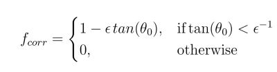
This optional argument can be accessed using the keyword step, and epsilon parameter must be specified. Another optional argument to specify the angular distribution of the products is the double keyword. In this option, the angular distribution on either sides of the peak are represented by a different cosine power decay. It requires one argument pol_pow_2, which describes the distribution between the peak and the surface. The distribution between the surface normal and the peak is described using the parameter pol_pow.
The keyword intenergy can be used to modify the internal energy of an incident molecule during collision. In the case of hyperthermal collision the energy from the translational mode is transfered to the internal modes. This keyword requires two input parameters frac_rot and frac_vib. These specify the fraction of the change in translational energy (difference between the final and initial) transferred to the rotational and vibrational mode respectively.
Output info:
All the surface collide models calculate a global vector of length 2. The values can be used by the stats_style command and by variables that define formulas. The latter means they can be used by any command that uses a variable as input, e.g. the fix ave/time command. See Section 4.4 for an overview of SPARTA output options.
The first element of the vector is the count of particles that hit surface elements assigned to this collision model during the current timestep. The second element is the cummulative count of particles that have hit surface elements since the current run began.
Styles with a kk suffix are functionally the same as the corresponding style without the suffix. They have been optimized to run faster, depending on your available hardware, as discussed in the Accelerating SPARTA section of the manual. The accelerated styles take the same arguments and should produce the same results, except for different random number, round-off and precision issues.
These accelerated styles are part of the KOKKOS package. They are only enabled if SPARTA was built with that package. See the Making SPARTA section for more info.
You can specify the accelerated styles explicitly in your input script by including their suffix, or you can use the -suffix command-line switch when you invoke SPARTA, or you can use the suffix command in your input script.
See the Accelerating SPARTA section of the manual for more instructions on how to use the accelerated styles effectively.
Restrictions:
The translate and rotate keywords cannot be used together.
If specified with a kk suffix, this command can be used no more than twice in the same input script (active at the same time).
Related commands:
Default:
The default for the temp/freq keyword = 1.
(Bird94) G. A. Bird, Molecular Gas Dynamics and the Direct Simulation of Gas Flows, Clarendon Press, Oxford (1994).
(Cercignani71) Cercignani C, Lampis M, Kinetic models for gas-surface interactions, Transport theory and statistical physics, Jan (1971).
(Lord90) R. G. Lord, presented at the 17th International Symposium on Rarefied Gas Dynamics, Germany, July (1990).
(Lord91) R. G. Lord, Some extensions of the Cercignani-Lampis gas-surface interaction model, Physics of Fluids A: Fluid Dynamics, Jan (1991).
(SG18) K. Swaminathan Gopalan, Development of a detailed surface chemistry framework in DSMC, AIAA Aerospace Sciences Meeting, Jan (2018).
(Rettner94a) C. T. Rettner, Reaction of an H-atom beam with Cl/Au(111): Dynamics of concurrent EleyRideal and Langmuir-Hinshelwood mechanisms, Journal of Chemical Physics, (1994).
(Alexander12) W. A. Alexander, et al, Kinematics and dynamics of atomic-beam scattering on liquid and self-assembled monolayer surfaces, Faraday discussions, (2012)
(Glatzer97) D. Glatzer, et al, Rotationally excited NO molecules incident on a graphite surface: in- and out-of-plane angular distributions, Surface Science, (1997)
(Lord95) R. G. Lord, Some further extensions of the Cercignani-Lampis gas-surface interaction model, Physics of Fluids, May (1995).
(Goodman72) F. O. Goodman, Simple model for the velocity distribution of molecules desorbed from surfaces following recombination of atoms, Surface Science, (1972).
(Rettner94b) C. T. Rettner and J. Lee, Dynamic displacement of o2 from pt (111): A new desorption mechanism, The Journal of chemical physics, (1994).
(Beckerle90) J. Beckerle, A. Johnson, and S. Ceyer, Collision-induced desorption of physisorbed CH4 from Ni (111): Experiments and simulations, The Journal of Chemical Physics, (1990).
(Goodman74) F. O. Goodman, Determination of characteristic surface vibration temperatures by molecular beam scattering: Application to specular scattering in the H-LiF (001) system, Surface Science, (1974).
(Mohammadzadeh16) A. Mohammadzadeh, A. Rana, and H. Struchtrup, DSMC and R13 modeling of the adiabatic surface, International Journal of Thermal Sciences, vol. 101, pp. 9–23, March (2016).