Syntax:
dump ID style mix-ID N file color diameter keyword value ...
  particle = yes/no = do or do not draw particles
  pdiam value = number = numeric value for particle diameter (distance units)
  grid values = color
    color = proc or per-grid compute or fix
  gridx values = xcoord color
    xcoord = x value to draw yz plane of grid cells at
    color = proc or per-grid compute or fix
  gridy values = ycoord color
    ycoord = y value to draw xz plane of grid cells at
    color = proc or per-grid compute or fix
  gridz values = zcoord color
    zcoord = z value to draw xy plane of grid cells at
    color = proc or per-grid compute or fix
  surf values = color diam
    color = one or proc or per-surf compute or fix
    diam = diameter of 2d lines as fraction of shortest box length
  size values = width height = size of images
    width = width of image in # of pixels
    height = height of image in # of pixels
  view values = theta phi = view of simulation box
    theta = view angle from +z axis (degrees)
    phi = azimuthal view angle (degrees)
    theta or phi can be a variable (see below)
  center values = flag Cx Cy Cz = center point of image
    flag = "s" for static, "d" for dynamic
    Cx,Cy,Cz = center point of image as fraction of box dimension (0.5 = center of box)
    Cx,Cy,Cz can be variables (see below)
  up values = Ux Uy Uz = direction that is "up" in image
    Ux,Uy,Uz = components of up vector
    Ux,Uy,Uz can be variables (see below)
  zoom value = zfactor = size that simulation box appears in image
    zfactor = scale image size by factor > 1 to enlarge, factor < 1 to shrink
    zfactor can be a variable (see below)
  persp value = pfactor = amount of "perspective" in image
    pfactor = amount of perspective (0 = none, < 1 = some, > 1 = highly skewed)
    pfactor can be a variable (see below)
  box values = yes/no diam = draw outline of simulation box
    yes/no = do or do not draw simulation box lines
    diam = diameter of box lines as fraction of shortest box length
  gline values = yes/no diam = draw outline of each grid cell
    yes/no = do or do not draw grid cell outlines
    diam = diameter of grid outlines as fraction of shortest box length
  sline values = yes/no diam = draw outline of each surface element
    yes/no = do or do not draw surf element outlines
    diam = diameter of surf element outlines as fraction of shortest box length
  axes values = yes/no length diam = draw xyz axes
    yes/no = do or do not draw xyz axes lines next to simulation box
    length = length of axes lines as fraction of respective box lengths
    diam = diameter of axes lines as fraction of shortest box length
  shiny value = sfactor = shinyness of spheres and cylinders
    sfactor = shinyness of spheres and cylinders from 0.0 to 1.0
  ssao value = yes/no seed dfactor = SSAO depth shading
    yes/no = turn depth shading on/off
    seed = random # seed (positive integer)
    dfactor = strength of shading from 0.0 to 1.0
Examples:
dump myDump image all 100 dump.*.jpg type type
dump myDump movie all 100 movie.mpg type type
These commands will dump shapshot images of all particles whose species are in the mix-ID to a file every 100 steps. The last two shell command will make a movie from the JPG files (once the run has finished) and play it in the Firefox browser:
dump                4 image all 100 tmp.*.jpg type type pdiam 0.2 view 90 -90
dump_modify	    4 pad 4
% convert tmp*jpg tmp.gif
% firefox tmp.gif
Description:
Dump a high-quality ray-traced image of the simulation every N timesteps and save the images either as a sequence of JPEG or PNG or PPM files, or as a single movie file. The options for this command as well as the dump_modify command control what is included in the image and how it appears.
Any or all of these entities can be included in the images:
Particles can be colored by any attribute allowed by the dump particle command. Grid cells and the x,y,z cutting planes can be colored by any per-grid attribute calculated by a compute or fix. Surface elements can be colored by any per-surf attribute calculated by a compute or fix.
A series of images can easily be converted into an animated movie of your simulation (see further details below), or the process can be automated without writing the intermediate files using the dump movie command. Other dump styles store snapshots of numerical data asociated with particles, grid cells, and surfaces in various formats, as discussed on the dump doc page.
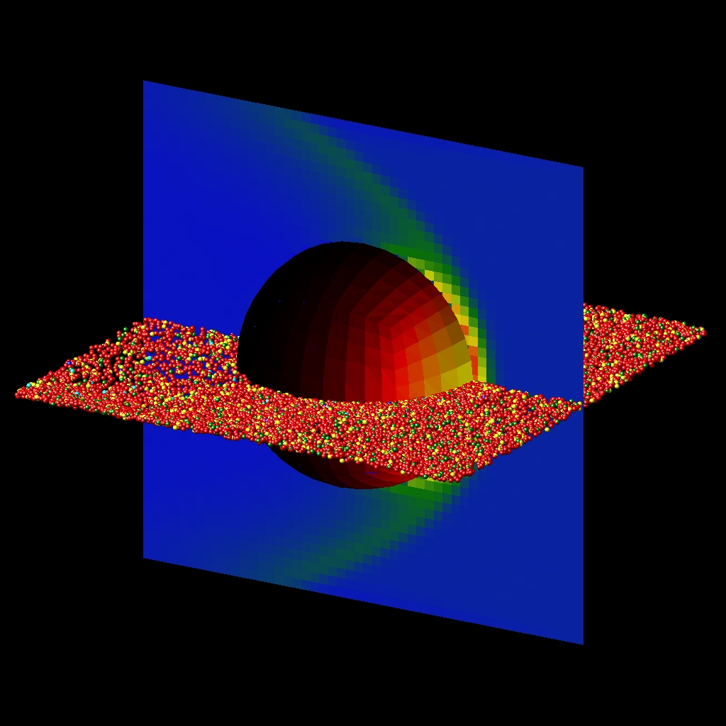
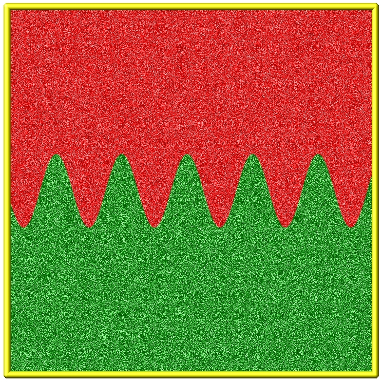
Here are two sample images, rendered as JPG files. Click to see the full-size images.
The left image is flow around a sphere with visualization of triangular surface elements on the sphere surface (colored by surface presssure), a vertical plane of grid cells (colored by particle density), and a horizontal plane of particles (colored by chemical species). The right image is the initial condition for a 2d simulation of Rayleigh-Taylor mixing as a relatively dense heavy gas (red) mixes with a light gas (green), driven by gravity in the downward direction.
The filename suffix determines whether a JPEG, PNG, or PPM file is created with the image dump style. If the suffix is ".jpg" or ".jpeg", then a JPEG format file is created, if the suffix is ".png", then a PNG format is created, else a PPM (aka NETPBM) format file is created. The JPEG and PNG files are binary; PPM has a text mode header followed by binary data. JPEG images have lossy compression; PNG has lossless compression; and PPM files are uncompressed but can be compressed with gzip, if SPARTA has been compiled with -DSPARTA_GZIP and a ".gz" suffix is used.
Similarly, the format of the resulting movie is chosen with the movie dump style. This is handled by the underlying FFmpeg converter program, which must be available on your machine, and thus details have to be looked up in the FFmpeg documentation. Typical examples are: .avi, .mpg, .m4v, .mp4, .mkv, .flv, .mov, .gif Additional settings of the movie compression like bitrate and framerate can be set using the dump_modify command.
To write out JPEG and PNG format files, you must build SPARTA with support for the corresponding JPEG or PNG library. To convert images into movies, SPARTA has to be compiled with the -DSPARTA_FFMPEG flag. See Section 2.2 of the manual for instructions on how to do this.
Dumps are performed on timesteps that are a multiple of N, including timestep 0. Note that this means a dump will not be performed on the initial timestep after the dump command is invoked, if the current timestep is not a multiple of N. This behavior can be changed via the dump_modify first command. N can be changed between runs by using the dump_modify every command.
Dump image filenames must contain a wildcard character "*", so that one image file per snapshot is written. The "*" character is replaced with the timestep value. For example, tmp.dump.*.jpg becomes tmp.dump.0.jpg, tmp.dump.10000.jpg, tmp.dump.20000.jpg, etc. Note that the dump_modify pad command can be used to insure all timestep numbers are the same length (e.g. 00010), which can make it easier to convert a series of images into a movie in the correct ordering.
Dump movie filenames on the other hand, must not have any wildcard character since only one file combining all images into a single movie will be written by the movie encoder.
Several of the keywords determine what objects are rendered in the image, namely particles, grid cells, or surface elements. There are additional optional kewords which control how the image is rendered. As listed below, all of the keywords have defaults, most of which you will likely not need to change. The dump modify also has options specific to the dump image style, particularly for assigning colors to particles and other image features.
Particles are drawn by default using the color and diameter settings. The particle keyword allow you to turn off the drawing of all particles, if the specified value is no.
Only particles in the specified mixture ID (mix-ID) are drawn. Only particles in a geometric region can be drawn using the dump_modify region command.
The color and diameter settings determine the color and size of particles rendered in the image. They can be any particle attribute defined for the dump particle command, including type.
The diameter setting can be overridden with a numeric value by the optional pdiam keyword, in which case you can specify the diameter setting with any valid particle attribute. The pdiam keyword overrides the diameter setting with a specified numeric value. All particles will be drawn with that diameter, e.g. 1.5, which is in whatever distance units the input script defines.
If type is specified for the color setting, then the color of each particle is determined by its type = species index. By default the mapping of types to colors is as follows:
and repeats itself for types > 6. This mapping can be changed by the dump_modify pcolor command.
If proc is specified for the color setting, then the color of each particle is determined by the ID of the owning processor. The default mapping of proc IDs to colors is that same as in the list above, except that proc P corresponds to type P+1.
If type is specified for the diameter setting then the diameter of each particle is determined by its type = species index. By default all types have diameter 1.0. This mapping can be changed by the dump_modify adiam command.
If proc is specified for the diameter setting then the diameter of each particle will be the proc ID (0 up to Nprocs-1) in whatever units you are using, which is undoubtably not what you want.
Any of the particle attributes listed in the dump custom command can also be used for the color or diameter settings. They are interpreted in the following way.
If "vx", for example, is used as the color setting, then the color of the particle will depend on the x-component of its velocity. The association of a per-particle value with a specific color is determined by a "color map", which can be specified via the dump_modify cmap command. The basic idea is that the particle-attribute will be within a range of values, and every value within the range is mapped to a specific color. Depending on how the color map is defined, that mapping can take place via interpolation so that a value of -3.2 is halfway between "red" and "blue", or discretely so that the value of -3.2 is "orange".
If "vx", for example, is used as the diameter setting, then the particle will be rendered using the x-component of its velocity as the diameter. If the per-particle value <= 0.0, them the particle will not be drawn.
The grid keyword turns on the drawing of grid cells with the specified color attribute. For 2d, the grid cell is shaded with an rectangle that is infinitely thin in the z dimension, which allows you to still see the particles in the grid cell. For 3d, the grid cell is drawn as a solid brick, which will obscure the particles inside it.
Only grid cells in a grid group can be drawn using the dump_modify gridgroup command. Only grid cells in a geometric region can be drawn using the dump_modify region command.
The gridx and gridy and gridz keywords turn on the drawing of of a 2d plane of grid cells at the specified coordinate. This is a way to draw one or more slices through a 3d image.
The dump_modify region command does not apply to the gridx and gridy and gridz plane drawing.
If proc is specified for the color setting, then the color of each grid cell is determined by its owning processor ID. This is useful for visualizing the result of a load balancing of the grid cells, e.g. by the balance_grid or fix balance commands. By default the mapping of proc IDs to colors is as follows:
and repeats itself for IDs > 6. Note that for this command, processor IDs range from 1 to Nprocs inclusive, instead of the more customary 0 to Nprocs-1. This mapping can be changed by the dump_modify gcolor command.
The color setting can also be a per-grid compute or fix. In this case, it is specified as c_ID or c_ID[N] for a compute and as f_ID and f_ID[N] for a fix.
This allows per grid cell values in a vector or array to be used to color the grid cells. The ID in the attribute should be replaced by the actual ID of the compute or fix that has been defined previously in the input script. See the compute or fix command for details.
If c_ID is used as a attribute, then the per-grid vector calculated by the compute is used. If c_ID[N] is used, then N must be in the range from 1-M, which will use the Nth column of the per-grid array calculated by the compute.
If f_ID is used as a attribute, then the per-grid vector calculated by the fix is used. If f_ID[N] is used, then N must be in the range from 1-M, which will use the Nth column of the per-grid array calculated by the fix.
The manner in which values in the vector or array are mapped to color is determined by the dump_modify cmap command.
The surf keyword turns on the drawing of surface elements with the specified color attribute. For 2d, the surface element is a line whose diameter is specified by the diam setting as a fraction of the minimum simulation box length. For 3d it is a triangle and the diam setting is ignored. The entire surface is rendered, which in 3d will hide any grid cells (or fractions of a grid cell) that are inside the surface.
Only surface elements in a surface group can be drawn using the dump_modify surfgroup command. The dump_modify region command does not apply to surface element drawing.
If one is specified for the color setting, then the color of every surface element is drawn with the color specified by the dump_modify scolor keyword, which is gray by default.
If proc is specified for the color setting, then the color of each surface element is determined by its owning processor ID. Surface elements are assigned to owning processors in a round-robin fashion. By default the mapping of proc IDs to colors is as follows:
and repeats itself for IDs > 6. Note that for this command, processor IDs range from 1 to Nprocs inclusive, instead of the more customary 0 to Nprocs-1. This mapping can be changed by the dump_modify scolor command, which has not yet been added to SPARTA.
The color setting can also be a per-surf compute or fix. In this case, it is specified as c_ID or c_ID[N] for a compute and as f_ID and f_ID[N] for a fix.
This allows per-surf values in a vector or array to be used to color the surface elemtns. The ID in the attribute should be replaced by the actual ID of the compute or fix that has been defined previously in the input script. See the compute or fix command for details.
If c_ID is used as a attribute, then the per-surf vector calculated by the compute is used. If c_ID[N] is used, then N must be in the range from 1-M, which will use the Nth column of the per-surf array calculated by the compute.
If f_ID is used as a attribute, then the per-surf vector calculated by the fix is used. If f_ID[N] is used, then N must be in the range from 1-M, which will use the Nth column of the per-surf array calculated by the fix.
The manner in which values in the vector or array are mapped to color is determined by the dump_modify cmap command.
The size keyword sets the width and height of the created images, i.e. the number of pixels in each direction.
The view, center, up, zoom, and persp values determine how 3d simulation space is mapped to the 2d plane of the image. Basically they control how the simulation box appears in the image.
All of the view, center, up, zoom, and persp values can be specified as numeric quantities, whose meaning is explained below. Any of them can also be specified as an equal-style variable, by using v_name as the value, where "name" is the variable name. In this case the variable will be evaluated on the timestep each image is created to create a new value. If the equal-style variable is time-dependent, this is a means of changing the way the simulation box appears from image to image, effectively doing a pan or fly-by view of your simulation.
The view keyword determines the viewpoint from which the simulation box is viewed, looking towards the center point. The theta value is the vertical angle from the +z axis, and must be an angle from 0 to 180 degrees. The phi value is an azimuthal angle around the z axis and can be positive or negative. A value of 0.0 is a view along the +x axis, towards the center point. If theta or phi are specified via variables, then the variable values should be in degrees.
The center keyword determines the point in simulation space that will be at the center of the image. Cx, Cy, and Cz are speficied as fractions of the box dimensions, so that (0.5,0.5,0.5) is the center of the simulation box. These values do not have to be between 0.0 and 1.0, if you want the simulation box to be offset from the center of the image. Note, however, that if you choose strange values for Cx, Cy, or Cz you may get a blank image. Internally, Cx, Cy, and Cz are converted into a point in simulation space. If flag is set to "s" for static, then this conversion is done once, at the time the dump command is issued. If flag is set to "d" for dynamic then the conversion is performed every time a new image is created. If the box size or shape is changing, this will adjust the center point in simulation space.
The up keyword determines what direction in simulation space will be "up" in the image. Internally it is stored as a vector that is in the plane perpendicular to the view vector implied by the theta and pni values, and which is also in the plane defined by the view vector and user-specified up vector. Thus this internal vector is computed from the user-specified up vector as
up_internal = view cross (up cross view)
This means the only restriction on the specified up vector is that it cannot be parallel to the view vector, implied by the theta and phi values.
The zoom keyword scales the size of the simulation box as it appears in the image. The default zfactor value of 1 should display an image mostly filled by the particles in the simulation box. A zfactor > 1 will make the simulation box larger; a zfactor < 1 will make it smaller. Zfactor must be a value > 0.0.
The persp keyword determines how much depth perspective is present in the image. Depth perspective makes lines that are parallel in simulation space appear non-parallel in the image. A pfactor value of 0.0 means that parallel lines will meet at infininty (1.0/pfactor), which is an orthographic rendering with no persepctive. A pfactor value between 0.0 and 1.0 will introduce more perspective. A pfactor value > 1 will create a highly skewed image with a large amount of perspective.
IMPORTANT NOTE: The persp keyword is not yet supported as an option.
The box keyword determines how the simulation box boundaries are rendered as thin cylinders in the image. If no is set, then the box boundaries are not drawn and the diam setting is ignored. If yes is set, the 12 edges of the box are drawn, with a diameter that is a fraction of the shortest box length in x,y,z (for 3d) or x,y (for 2d). The color of the box boundaries can be set with the dump_modify boxcolor command.
The gline keyword determines how the outlines of grid cells are rendered as thin cylinders in the image. If the gridx or gridy or gridz keywords are specified to draw a plane(s) of grid cells, then outlines of all cells in the plane(s) are drawn. If the planar options are not used, then the outlines of all grid cells are drawn, whether the grid keyword is specified or not. In this case, the dump_modify region command can be used to restrict which grid cells the outlines are drawn for.
For the gline keywork, if no is set, then grid outlines are not drawn and the diam setting is ignored. If yes is set, the 12 edges of each grid cell are drawn, with a diameter that is a fraction of the shortest box length in x,y,z (for 3d) or x,y (for 2d). The color of the grid cell outlines can be set with the dump_modify glinecolor command.
The sline keyword determines how the outlines of surface elements are rendered as thin cylinders in the image. If no is set, then the surface element outlines are not drawn and the diam setting is ignored. If yes is set, a line is drawn for 2d and a triangle outline for 3d surface elements, with a diameter that is a fraction of the shortest box length in x,y,z (for 3d) or x,y (for 2d). The color of the surface element outlines can be set with the dump_modify slinecolor command.
The axes keyword determines how the coordinate axes are rendered as thin cylinders in the image. If no is set, then the axes are not drawn and the length and diam settings are ignored. If yes is set, 3 thin cylinders are drawn to represent the x,y,z axes in colors red,green,blue. The origin of these cylinders will be offset from the lower left corner of the box by 10%. The length setting determines how long the cylinders will be as a fraction of the respective box lengths. The diam setting determines their thickness as a fraction of the shortest box length in x,y,z (for 3d) or x,y (for 2d).
The shiny keyword determines how shiny the objects rendered in the image will appear. The sfactor value must be a value 0.0 <= sfactor <= 1.0, where sfactor = 1 is a highly reflective surface and sfactor = 0 is a rough non-shiny surface.
The ssao keyword turns on/off a screen space ambient occlusion (SSAO) model for depth shading. If yes is set, then particles further away from the viewer are darkened via a randomized process, which is perceived as depth. The calculation of this effect can increase the cost of computing the image by roughly 2x. The strength of the effect can be scaled by the dfactor parameter. If no is set, no depth shading is performed.
A series of JPEG, PNG, or PPM images can be converted into a movie file and then played as a movie using commonly available tools. Using dump style movie automates this step and avoids the intermediate step of writing (many) image snapshot file.
To manually convert JPEG, PNG or PPM files into an animated GIF or MPEG or other movie file you can:
% convert *.jpg foo.gif
% convert -loop 1 *.ppm foo.mpg
Animated GIF files from ImageMagick are unoptimized. You can use a program like gifsicle to optimize and massively shrink them. MPEG files created by ImageMagick are in MPEG-1 format with rather inefficient compression and low quality.
Select "Open Image Sequence" under the File menu Load the images into QuickTime to animate them Select "Export" under the File menu Save the movie as a QuickTime movie (*.mov) or in another format. QuickTime can generate very high quality and efficiently compressed movie files. Some of the supported formats require to buy a license and some are not readable on all platforms until specific runtime libraries are installed.
FFmpeg is a command line tool that is available on many platforms and allows extremely flexible encoding and decoding of movies.
cat snap.*.jpg | ffmpeg -y -f image2pipe -c:v mjpeg -i - -b:v 2000k movie.m4v
cat snap.*.ppm | ffmpeg -y -f image2pipe -c:v ppm -i - -b:v 2400k movie.avi
Frontends for FFmpeg exist for multiple platforms. For more information see the FFmpeg homepage
You can play a movie file as follows:
Select "Open File" under the File menu Load the animated GIF file
% mplayer foo.mpg
% ffplay bar.avi
a = animate("foo*.jpg")
Restrictions:
To write JPEG images, you must use the -DSPARTA_JPEG switch when building SPARTA and link with a JPEG library. To write PNG images, you must use the -DSPARTA_PNG switch when building SPARTA and link with a PNG library.
To write movie files, you must use the -SPARTA_FFMPEG switch when building SPARTA. The FFmpeg executable must also be available on the machine where SPARTA is being run. Typically it's name is lowercase, i.e. ffmpeg.
See Section 2.2.2 section of the documentation for details on how to compile with optional switches.
Note that since FFmpeg is run as an external program via a pipe, SPARTA has limited control over its execution and no knowledge about errors and warnings printed by it. Those warnings and error messages will be printed to the screen only. Due to the way image data is communicated to FFmpeg, it will often print the message + pipe:: Input/output error :pre + which can be safely ignored. Other warnings and errors have to be addressed according to the FFmpeg documentation. One known issue is that certain movie file formats (e.g. MPEG level 1 and 2 format streams) have video bandwith limits that can be crossed when rendering too large of image sizes. Typical warnings look like this:
[mpeg @ 0x98b5e0] packet too large, ignoring buffer limits to mux it
[mpeg @ 0x98b5e0] buffer underflow st=0 bufi=281407 size=285018
[mpeg @ 0x98b5e0] buffer underflow st=0 bufi=283448 size=285018
In this case it is recommended to either reduce the size of the image or encode in a different format that is also supported by your copy of FFmpeg, and which does not have this limitation (e.g. .avi, .mkv, mp4).
Related commands:
Default:
The defaults for the keywords are as follows: