Syntax:
balance_grid style args ...
  none args = none
  stride args = xyz or xzy or yxz or yzx or zxy or zyx
  clump args = xyz or xzy or yxz or yzx or zxy or zyx
  block args = Px Py Pz
    Px,Py,Pz = # of processors in each dimension
  random args = none
  proc args = none
  rcb args = weight
    weight = cell or part or time
  axes value = dims
    dims = string with any of "x", "y", or "z" characters in it
  flip value = yes or no
Examples:
balance_grid block * * *
balance_grid block * 4 *
balance_grid clump yxz
balance_grid random
balance_grid rcb part
balance_grid rcb part axes xz
Description:
This command adjusts the assignment of grid cells and their particles to processors, to attempt to balance the computational cost (load) evenly across processors. The load balancing is "static" in the sense that this command performs the balancing once, before or between simulations. The assignments will remain static during the subsequent run. To perform "dynamic" balancing, see the fix balance command, which can adjust the assignemt of grid cells to processors on-the-fly during a run.
After grid cells have been assigned, they are migrated to new owning processors, along with any particles they own or other per-cell attributes stored by fixes. The internal data structures within SPARTA for grid cells and particles are re-initialized with the new decomposition.
This command can be used immediately after the grid is created, via the create_grid or read_restart commands. In the former case balance_grid can be used to partition the grid in a more desirable manner than the default creation options allow for. In the latter case, balance grid can be used to change the somewhat random assignment of grid cells to processors that will be made if the restart file is read by a different number of processors than it was written by.
This command can also be used once particles have been created, or a simulation has come to equilibrium with a spatially varying density distribution of particles, so that the computational load is more evenly balanced across processors.
The details of how child cells are assigned to processors by the various options of this command are described below. The cells assigned to each processor will either be "clumped" or "dispersed".
The clump and block and rcb styles will produce clumped assignments of child cells to each processor. This means each processor's cells will be geometrically compact. The stride and random and proc styles will produce dispersed assignments of child cells to each processor.
IMPORTANT NOTE: See Section 6.8 of the manual for an explanation of clumped and dispersed grid cell assignments and their relative performance trade-offs.
The none style will not change the assignment of grid cells to processors. However it will update the internal data structures within SPARTA that store ghost cell information on each processor for cells owned by other processors. This is useful if the global gridcut command was used after grid cells were already defined. That command erases ghost cell information stored by processors, which then needs to be re-generated before a simulation is run. Using the balance_grid none command will re-generate the ghost cell information.
The stride, clump, and block styles can only be used if the grid is "uniform". The grid in SPARTA is hierarchical with one or more levels, as defined by the create_grid or read_grid commlands. If the parent cell of every grid cell is at the same level of the hierarchy, then for purposes of this command the grid is uniform, meaning the collection of grid cells effectively form a uniform fine grid overlaying the entire simulation domain.
The meaning of the stride, clump, and block styles is exactly the same as when they are used as keywords with the create_grid command. See its doc page for details.
The random style means that each grid cell will be assigned randomly to one of the processors. Note that in this case every processor will typically not be assigned the exact same number of cells.
The proc style means that each processor will choose a random processor to assign its first grid cell to. It will then loop over its grid cells and assign each to consecutive processors, wrapping around the enumeration of processors if necessary. Note that in this case every processor will typically not be assigned exactly the same number of cells.
The rcb style uses a recursive coordinate bisectioning (RCB) algorithm to assign spatially-compact clumps of grid cells to processors. Each grid cell has a "weight" in this algorithm so that each processor is assigned an equal total weight of grid cells, as nearly as possible.
If the weight argument is specified as cell, then the weight for each grid cell is 1.0, so that each processor will end up with an equal number of grid cells.
If the weight argument is specified as part, then the weight for each grid cell is the number of particles it currently owns, so that each processor will end up with an equal number of particles.
If the weight argument is specified as time, then timers are used to estimate the cost of each grid cell. The cost from the timers is given on a per processor basis, and then assigned to grid cells by weighting by the relative number of particles in the grid cells. If no timing data has yet been collected at the point in a script where this command is issued, a cell style weight will be used instead of time. A small warmup run (for example 100 timesteps) can be used before the balance command so that timer data is available. The timers used for balancing tally time from the move, sort, collide, and modify portions of each timestep.
IMPORTANT NOTE: The adapt_grid command zeros out timing data, so the weight time option is not available immediatly after this command.
IMPORTANT NOTE: The coarsening option in fix_adapt may shift cells to different processors, which makes the accumulated timing data for the weight time option less accurate when load balancing is performed immediately after this command.
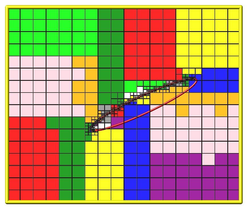
Here is an example of an RCB partitioning for 24 processors, of a 2d hierarchical grid with 5 levels, refined around a tilted ellipsoidal surface object (outlined in pink). This is for a weight cell setting, yielding an equal number of grid cells per processor. Each processor is assigned a different color of grid cells. (Note that less colors than processors were used, so the disjoint yellow cells actually belong to three different processors). This is an example of a clumped distribution where each processor's assigned cells can be compactly bounded by a rectangle. Click for a larger version of the image.
The optional keywords axes and flip only apply to the rcb style. Otherwise they are ignored.
The axes keyword allows limiting the partitioning created by the RCB algorithm to a subset of dimensions. The default is to allow cuts in all dimension, e.g. x,y,z for 3d simulations. The dims value is a string with 1, 2, or 3 characters. The characters must be one of "x", "y", or "z". They can be in any order and must be unique. For example, in 3d, a dims = xz would only partition the 3d grid only in the x and z dimensions.
The flip keyword is useful for debugging. If it is set to yes then each time an RCB partitioning is done, the coordinates of grid cells will (internally only) undergo a sign flip to insure that the new owner of each grid cell is a different processor than the previous owner, at least when more than a few processors are used. This will insure all particle and grid data moves to new processors, fully exercising the rebalancing code.
Restrictions:
This command can only be used after the grid has been created by the create_grid, read_grid, or read_restart commands.
This command also initializes various options in SPARTA before performing the balancing. This is so that grid cells are ready to migrate to new processors. Thus if an error is flagged, e.g. that a simulation box boundary condition is not yet assigned, that operation needs to be performed in the input script before balancing can be performed.
Related commands:
Default:
The default settings for the optional keywords are axes = xyz, flip = no.