SPARTA Benchmarks

This page gives SPARTA performance on several benchmark problems, run on different machines, both in serial and parallel. When the hardware supports it, results using the the accelerator options currently available in the code are also shown.

All the information is provided below to run these tests or similar tests on your own machine. This includes info on how to build SPARTA, how to launch it with the appropriate command-line arguments, and links to input and output files generated by all the benchmark tests. Note that input files and a few sample output files are also provided in the bench directory of the SPARTA distribution. See the bench/README file for details.

Benchmark results:

• Free = free molecular flow in a box, older results on a large BG/Q machine
• Collide = collisional molecular flow in a box , older results on a large BG/Q machine
• Free = same as above, with accelerator options and new machines
• Collide = same as above, with accelerator options and new machines
• Sphere = flow around a sphere, with accelerator options and new machines

Additional info:

• Accelerator options
• Machines and node hardware
• How to build SPARTA and run the benchmarks
• How to interpret the plots

Free molecular flow in a box

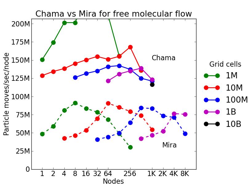
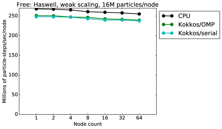
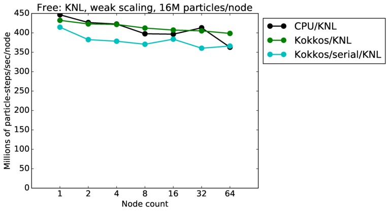
This benchmark is for particles advecting in free molecular flow (no collsions) on a regular grid overlaying a 3d closed box with reflective boundaries. The size of the grid was varied; the particle counts is always 10x the number of grid cells. Particles were initialized with a thermal temperature (no streaming velocity) so they move in random directions. Since there is very little computation to do, this is a good stress test of the communication capabilities of SPARTA and the machines it is run on.

The input script for this problem is bench/in.free in the SPARTA distribution.

This plot shows timings results in particle moves/sec/node, for runs of different sizes on varying node counts of two different machines. Problems as small as 1M grid cells (10M particles) and as large as 10B grid cells (100B particles) were run.

Chama is an Intel cluster with Infiniband described below. Each node of chama has dual 8-core Intel Sandy Bridge CPUs. These tests were run on all 16 cores of each node, i.e. with 16 MPI tasks/node. Up to 1024 nodes were used (16K MPI tasks). Mira is an IBM BG/Q machine at Argonne National Labs. It has 16 cores per node. These tests were run with 4 MPI tasks/core, for a total of 64 MPI tasks/node. Up to 8K nodes were used (512K MPI tasks).

The plot shows that a Chama node is about 2x faster than a BG/Q node.

Each individual curve in the plot is a strong scaling test, where the same size problem is run on more and more nodes. Perfect scalability would be a horizontal line. The curves show some initial super-linear speed-up as the particle count/node decreased, due to cache effects, then a slow-down as more nodes are added due to too-few particles/node and increased communication costs.

Jumping from curve-to-curve as node count increases is a weak scaling test, since the problem size is increasing with node count. Again a horizontal line would represent perfect weak scaling.

Click on the image to see a larger version.

Collisional flow in a box

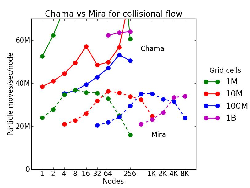
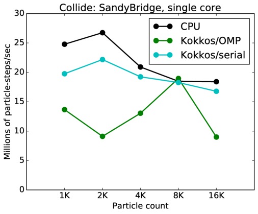
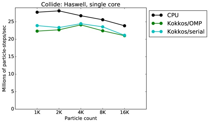
This benchmark is for particles undergoing collisional flow. Everything about the problem is the same as the free molecular flow problem described above, except that collisions were enabled, which requires extra computation, as well as particle sorting each timestep to identify particles in the same grid cell.

The input script for this problem is bench/in.collide in the SPARTA distribution.

As above, this plot shows timings results in particle moves/sec/node, for runs of different sizes on varying node counts. Data for the same two machines is shown: chama (Intel cluster with Ifiniband at Sandia) and mira (IBM BG/Q at ANL). Comparing these timings to the free molecule flow plot in the previous section shows the cost of collisions (and sorting) slows down the performance by a factor of about 2.5x. Cache effects (super-linear speed-up) are smaller due to the increased computational costs.

For collisional flow, problems as small as 1M grid cells (10M particles) and as large as 1B grid cells (10B particles) were run.

The discussion above regarding strong and weak scaling also applies to this plot. For any curve, a horizontal line would represent perfect weak scaling.

Click on the image to see a larger version.

Free benchmark

• in.free input script

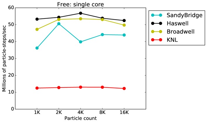
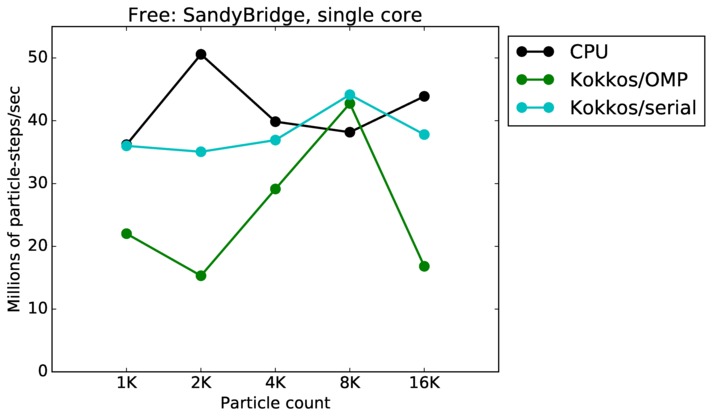
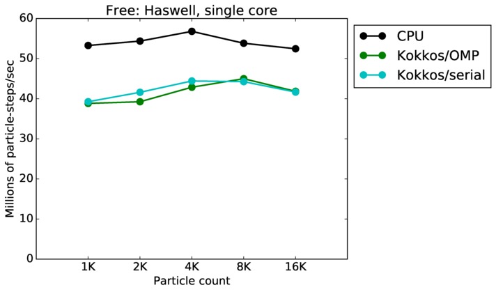
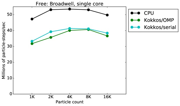
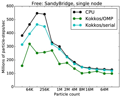
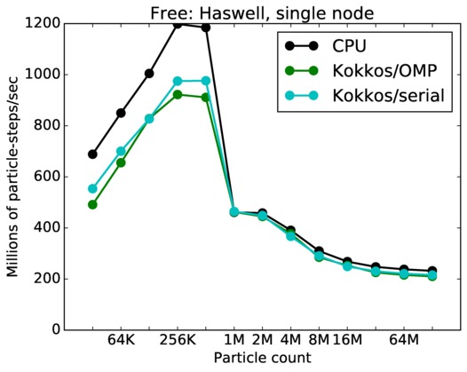
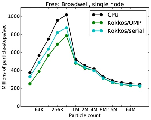
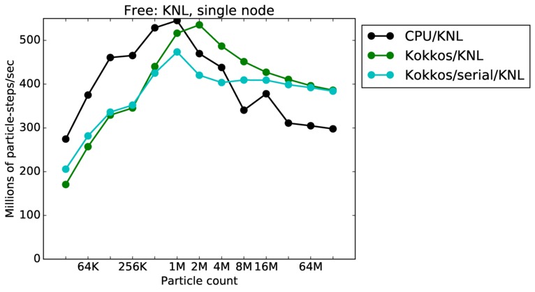
As described above, this benchmark is for particles advecting in free molecular flow (no collisions) on a regular grid overlaying a 3d closed box with reflective boundaries. The size of the grid was varied; the particle counts is always 10x the number of grid cells. Particles were initialized with a thermal temperature (no streaming velocity) so they move in random directions. Since there is very little computation to do, this is a good stress test of the communication capabilities of SPARTA and the machines it is run on.

Additional packages needed for this benchmark: none

Comments:

• In the data below, K = 1000 particles, so 1M = 1024*1000.

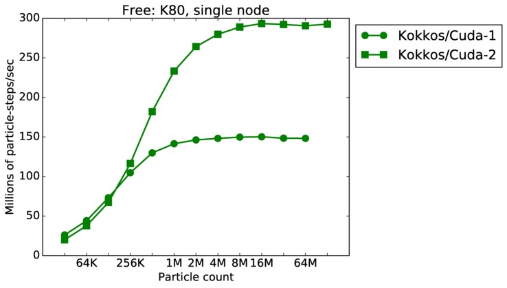
Free single core and single node performance:

Best timings for any accelerator option as a function of problem size. Running on a single CPU or KNL core. Running on a single CPU or KNL node or a single GPU. Only for double precision.

• Table for single core
• Table for single node

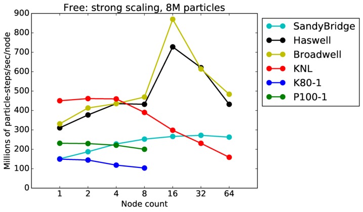
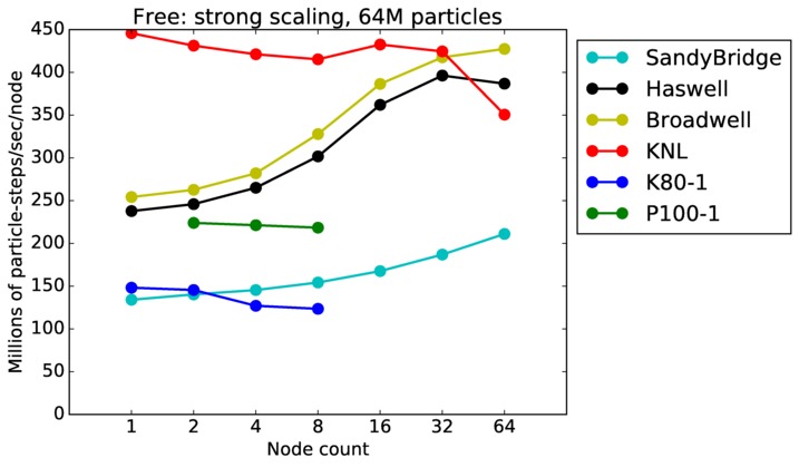
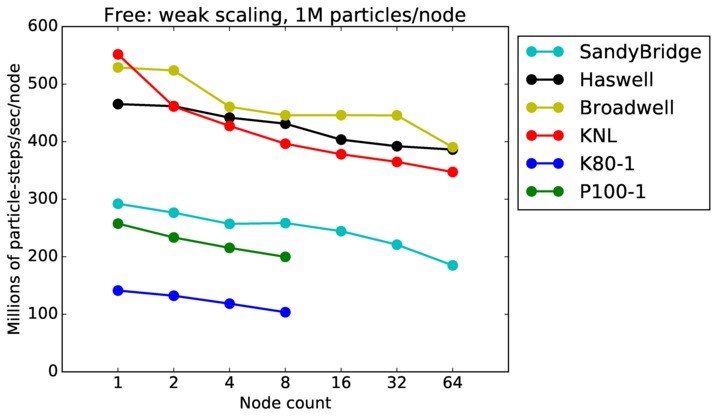
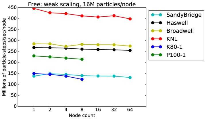
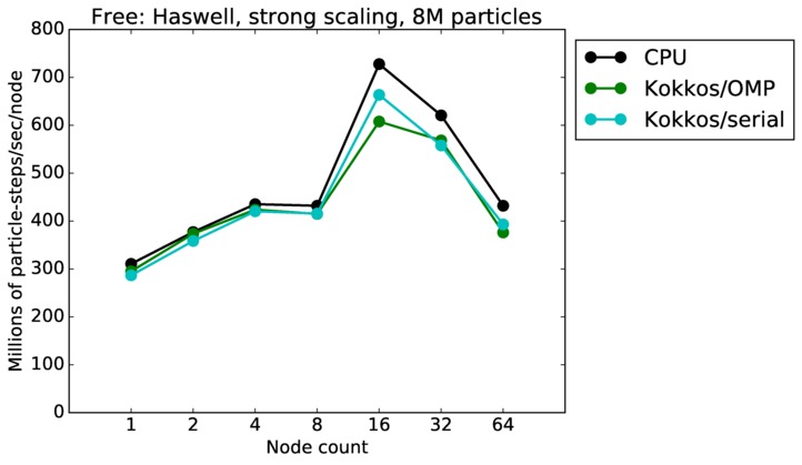
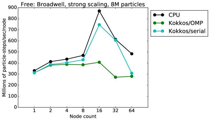
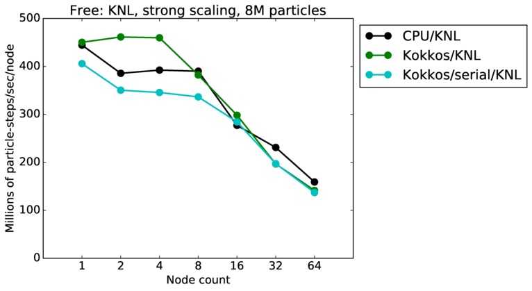
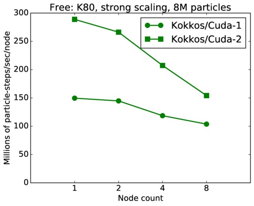
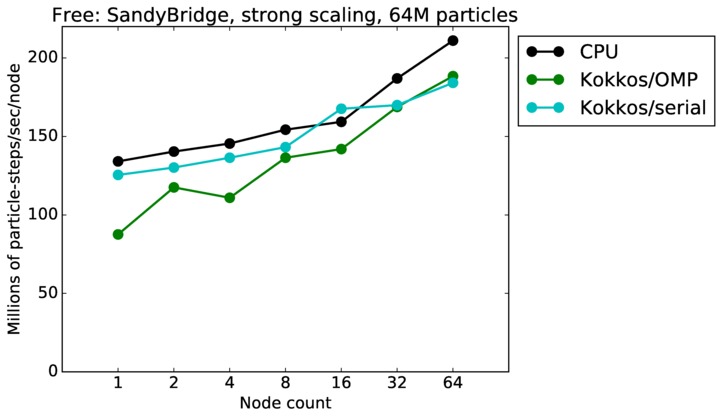
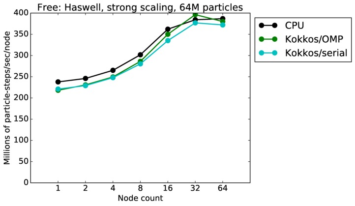
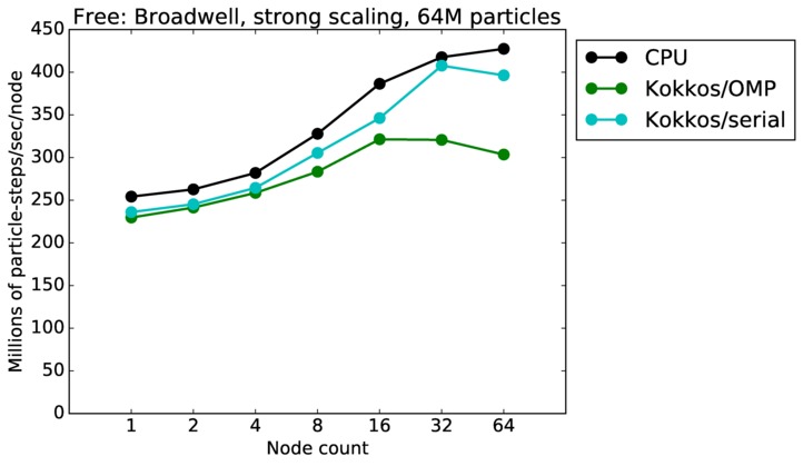
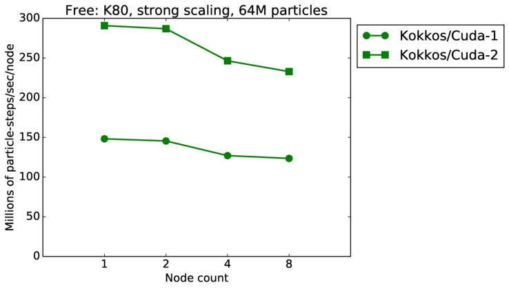
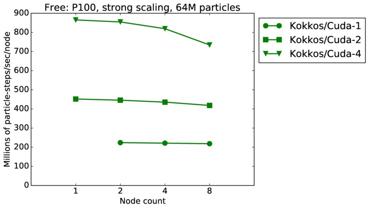
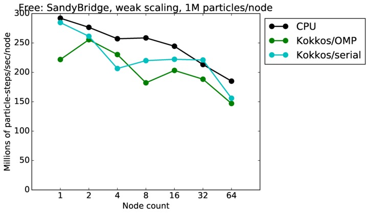
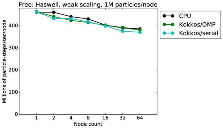
Free strong and weak scaling:

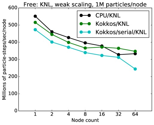
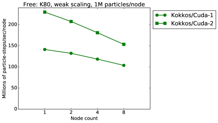
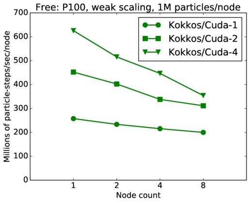
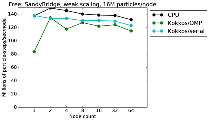
Fastest timing for any accelerator option running on multiple CPU or KNL or a single GPUs, as a function of node count. For strong scaling of 2 problem sizes: 8M particles, 64M particles. For weak scaling of 2 problem sizes: 1M particles/node, 16M particles/node. Only for a single GPU/node, only double precision.

Strong scaling means the same size problem is run on successively more nodes. Weak scaling means the problem size doubles each time the node count doubles. See a fuller description here of how to interpret these plots.

• Table for strong scaling of 8M particles
• Table for strong scaling of 64M particles
• Table for weak scaling of 1M particles/node
• Table for weak scaling of 16M particles/node

Free performance details:

• Modes: per-core, per-node, strong scaling, weak scaling
• Hardware: CPU, KNL, GPU options
• Within plot: accelerator packages, one or multiple GPUs/node

Collide benchmark

• in.collide input script
• in.collide.kokkos_cuda variant for Kokkos/Cuda package

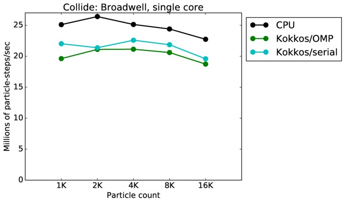
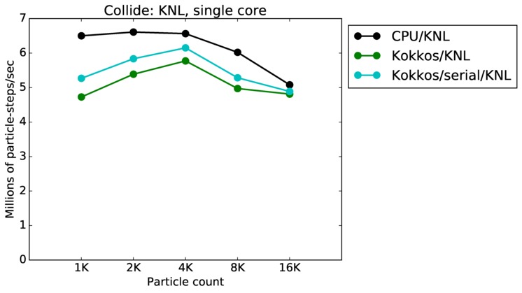
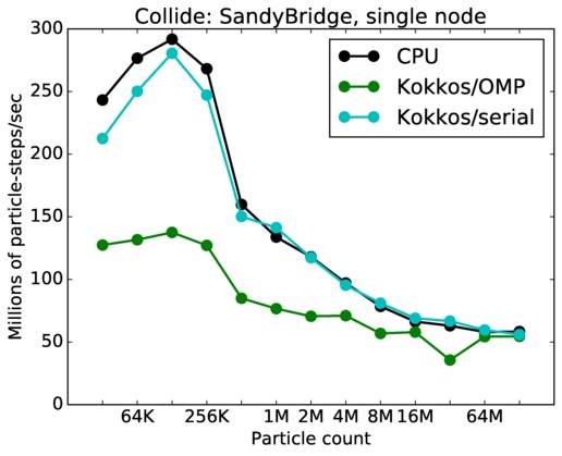
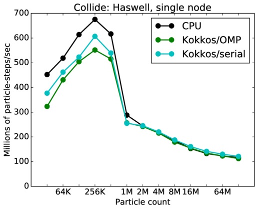
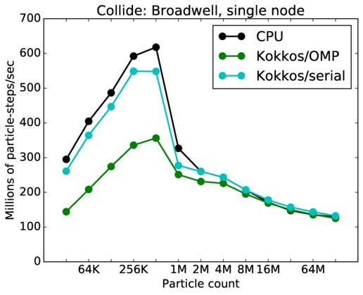
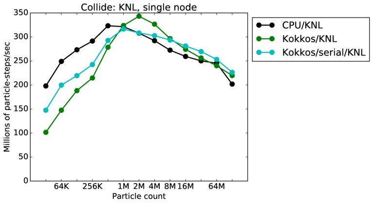
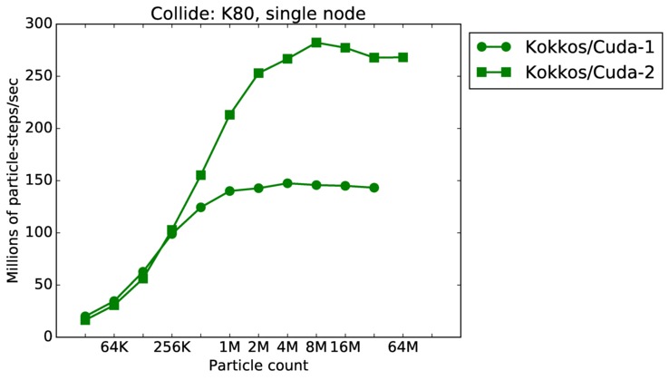
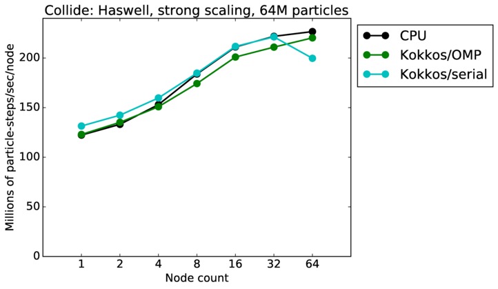
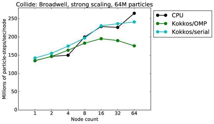
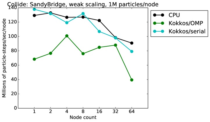
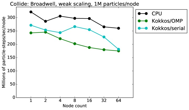
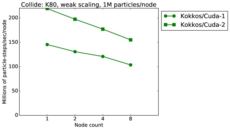
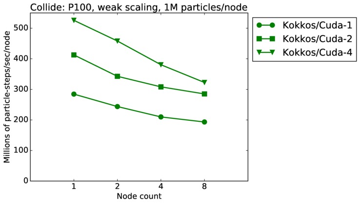
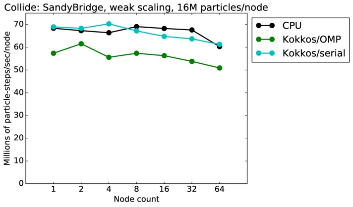
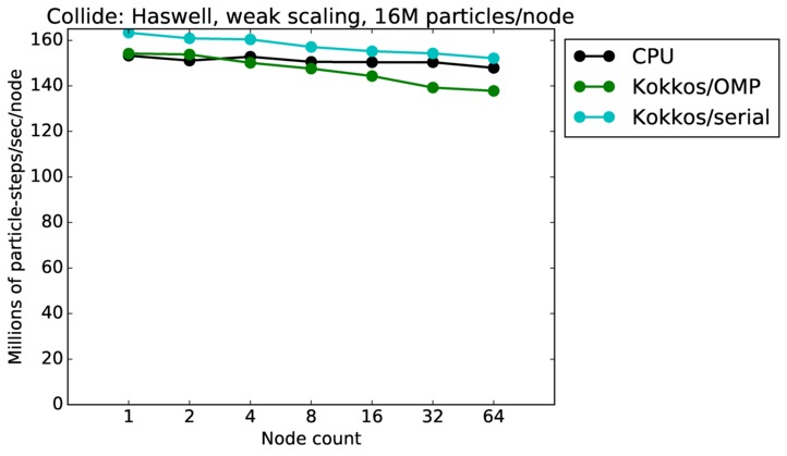
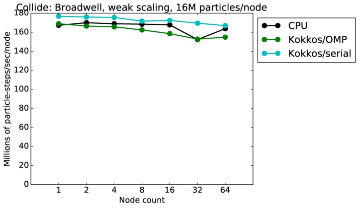
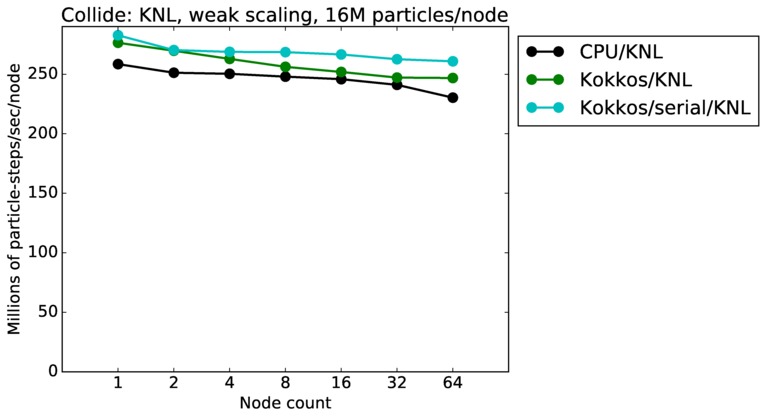
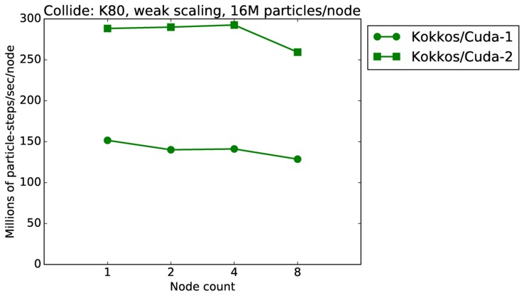
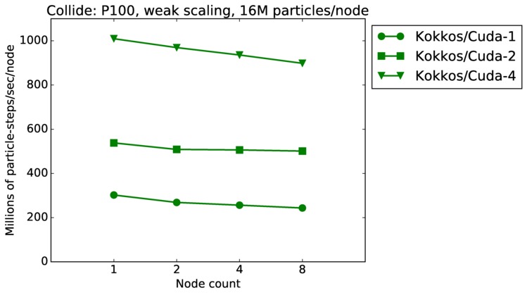
As described above, this benchmark is for particles undergoing collisional flow. Everything about the problem is the same as the free molecular flow problem described above, except that collisions were enabled, which requires extra computation, as well as particle sorting each timestep to identify particles in the same grid cell.

Additional packages needed for this benchmark: none

Comments:

• In the data below, K = 1000 particles, so 1M = 1024*1000.

Collide single core and single node performance:

Best timings for any accelerator option as a function of problem size. Running on a single CPU or KNL core. Running on a single CPU or KNL or a single GPU. Only for double precision.

• Table for single core
• Table for single node

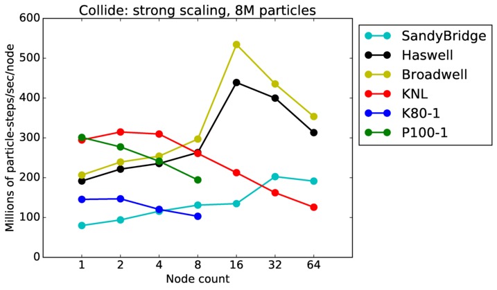
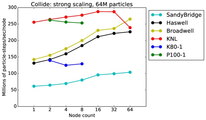
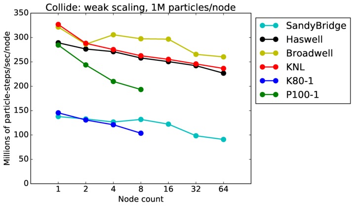
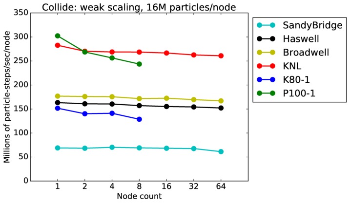
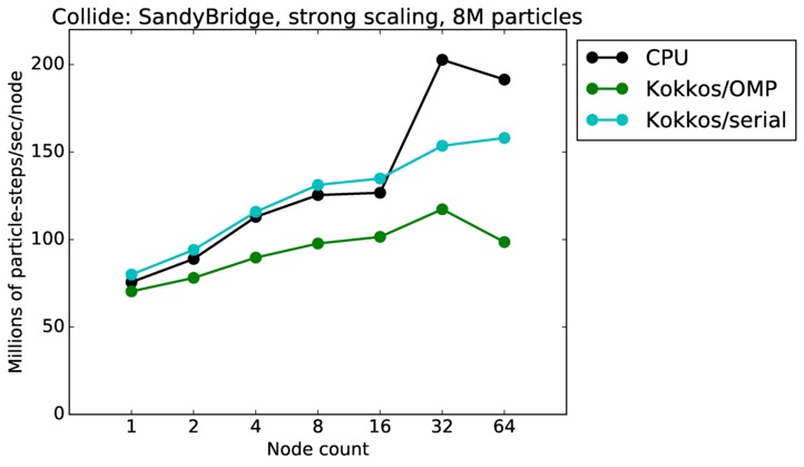
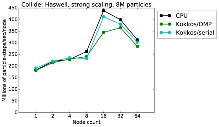
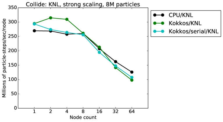
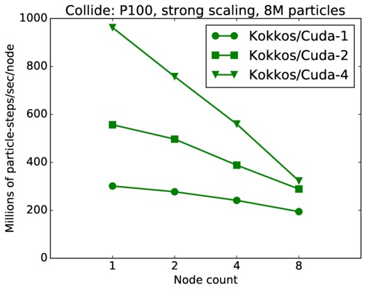
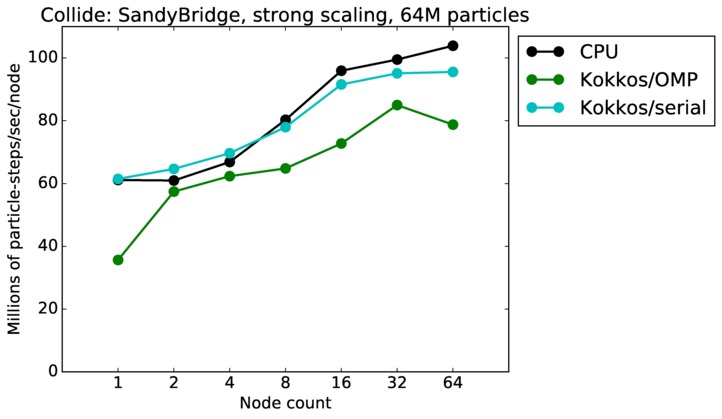
Collide strong and weak scaling:

Fastest timing for any accelerator option running on multiple CPU or KNL or a single GPUs, as a function of node count. For strong scaling of 2 problem sizes: 8M particles, 64M particles. For weak scaling of 2 problem sizes: 1M particles/node, 16M particles/node. Only for a single GPU/node, only double precision.

Strong scaling means the same size problem is run on successively more nodes. Weak scaling means the problem size doubles each time the node count doubles. See a fuller description here of how to interpret these plots.

• Table for strong scaling of 8M particles
• Table for strong scaling of 64M particles
• Table for weak scaling of 1M particles/node
• Table for weak scaling of 16M particles/node

Collide performance details:

• Modes: per-core, per-node, strong scaling, weak scaling
• Hardware: CPU, KNL, GPU options
• Within plot: accelerator packages, one or multiple GPUs/node

Sphere benchmark

• in.sphere input script
• in.sphere.kokkos_cuda variant for Kokkos/Cuda package

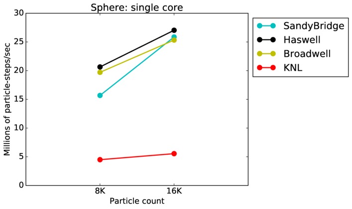
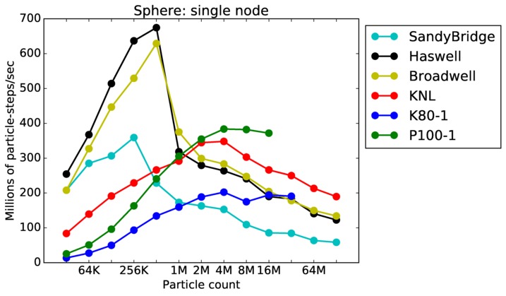
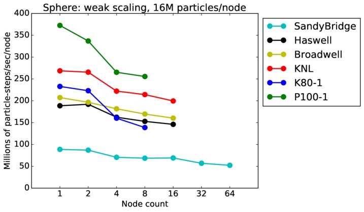
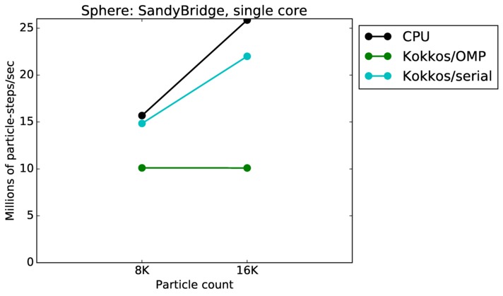
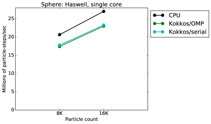
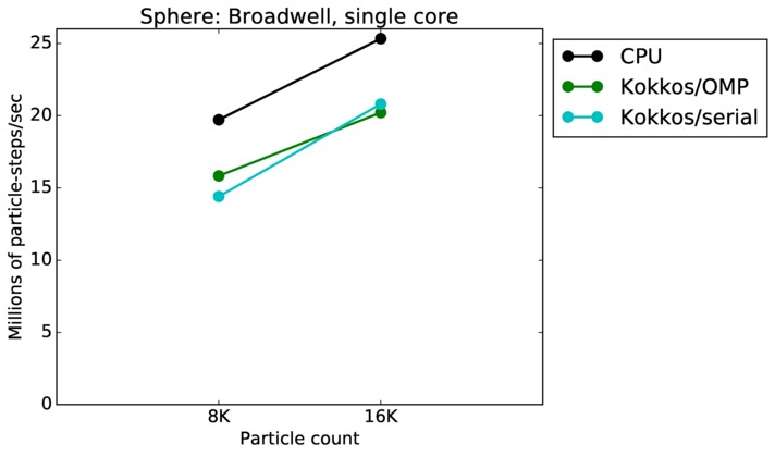
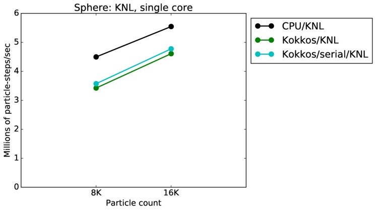
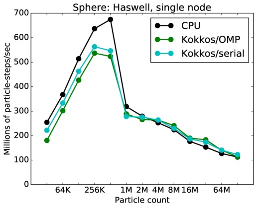
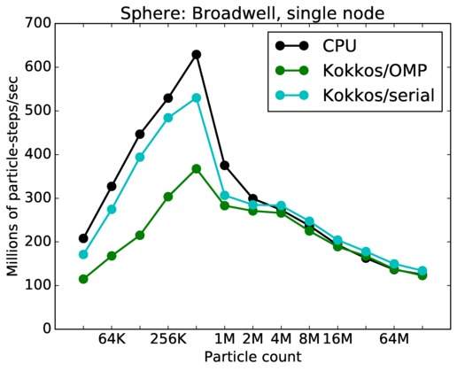
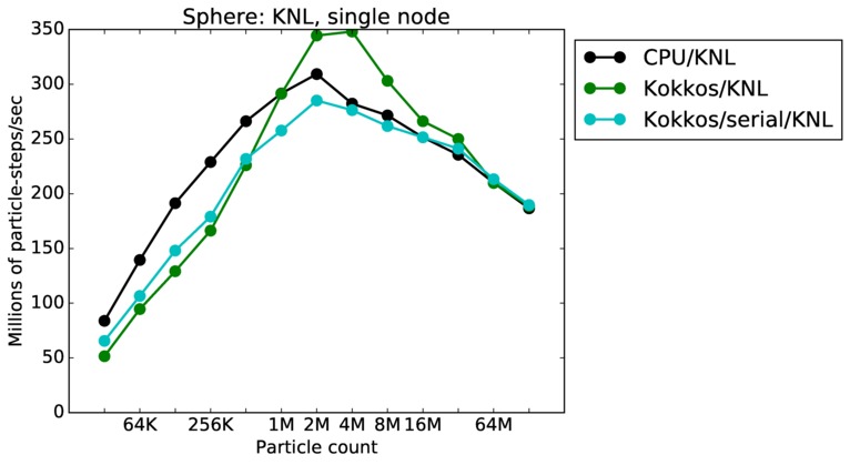
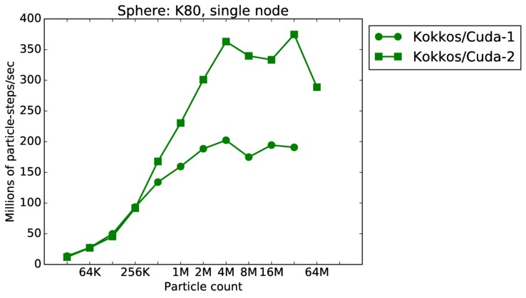
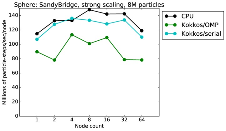
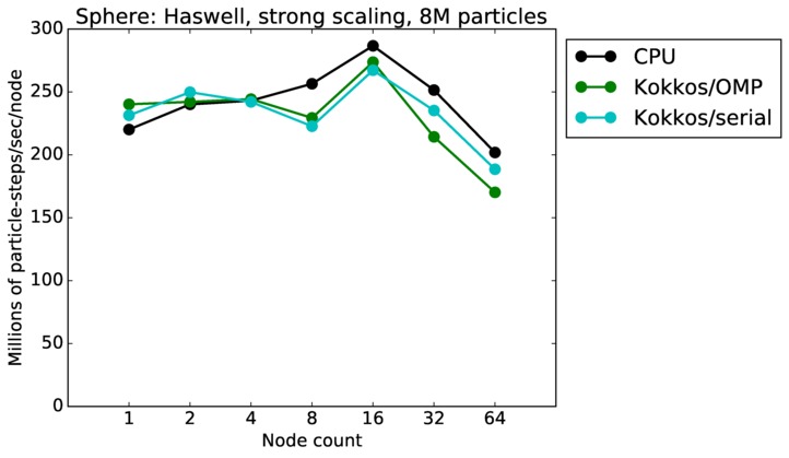
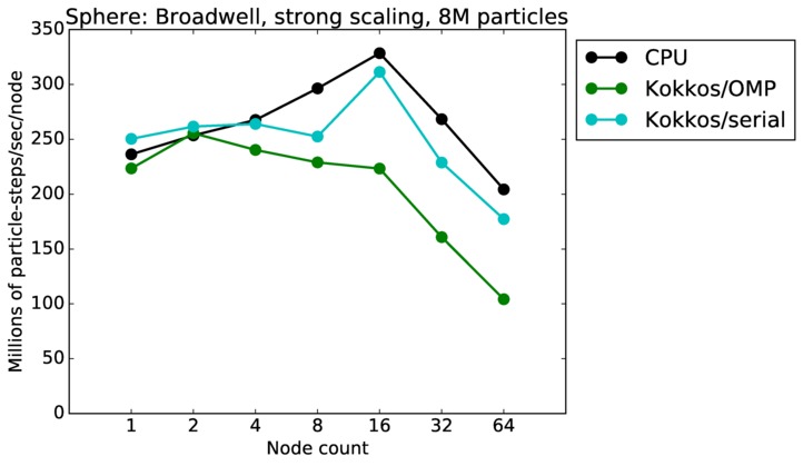
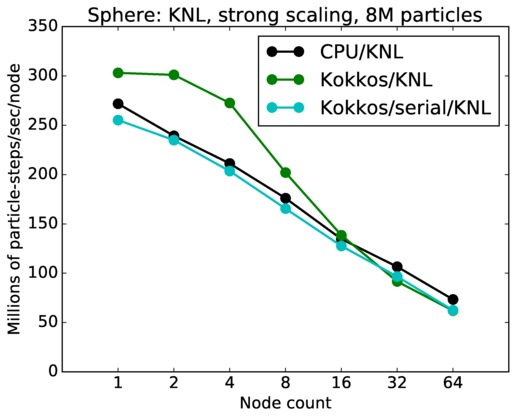
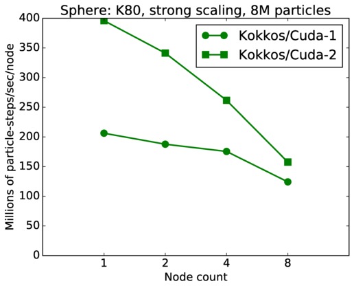
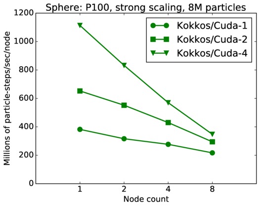
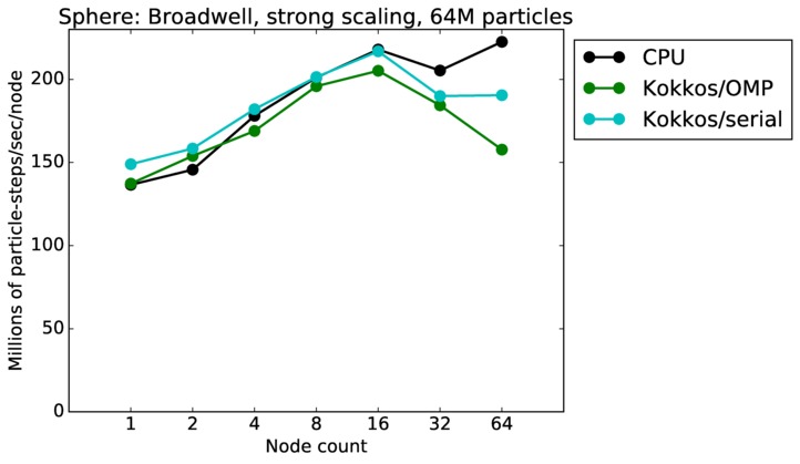
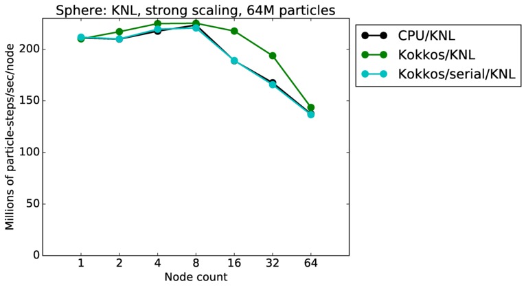
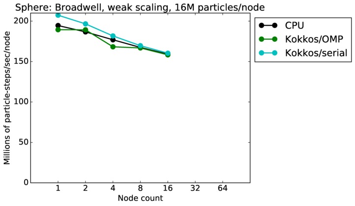
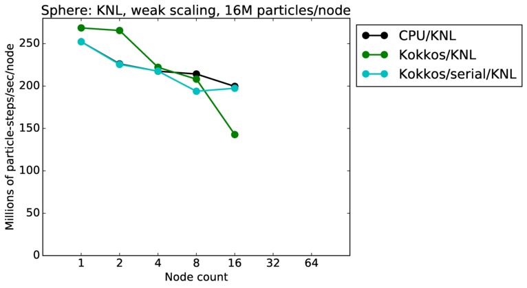
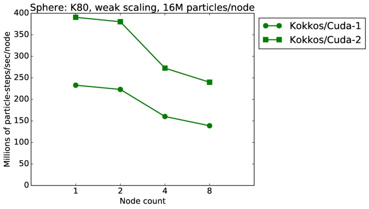
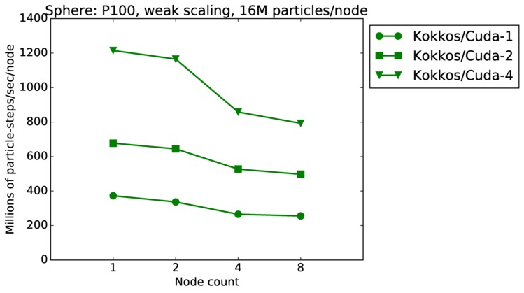
This benchmark is for particles flowing around a sphere.

Comments:

• In the data below, K = 1000 particles, so 1M = 1024*1000.

Sphere single core and single node performance:

Best timings for any accelerator option as a function of problem size. Running on a single CPU or KNL core. Running on a single CPU or KNL node or a single GPU. Only for double precision.

• Table for single core
• Table for single node

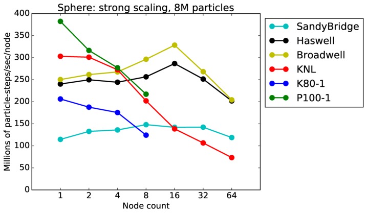
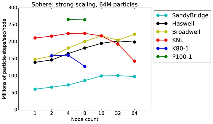
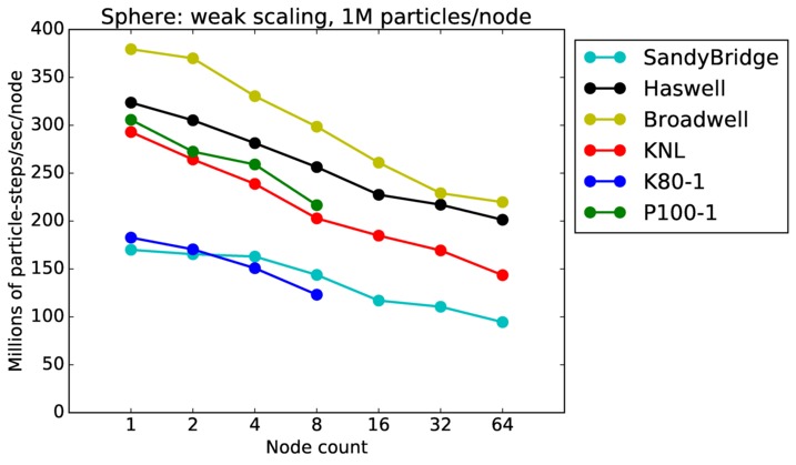
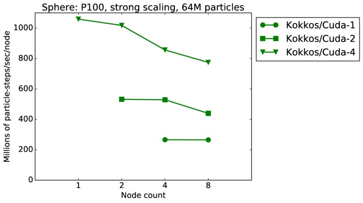
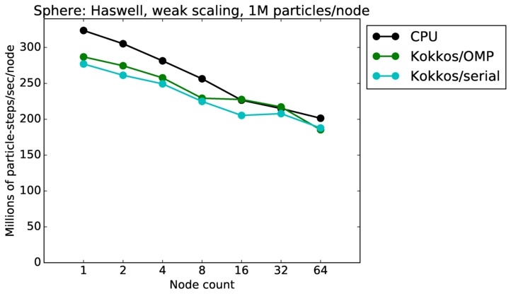
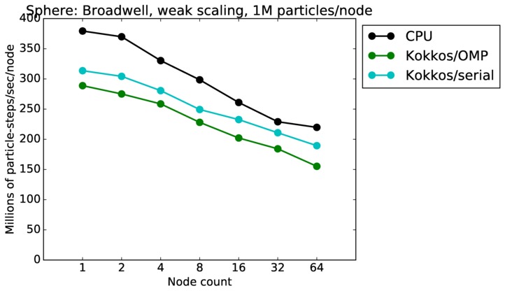
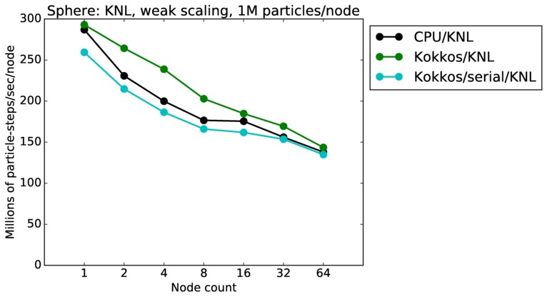
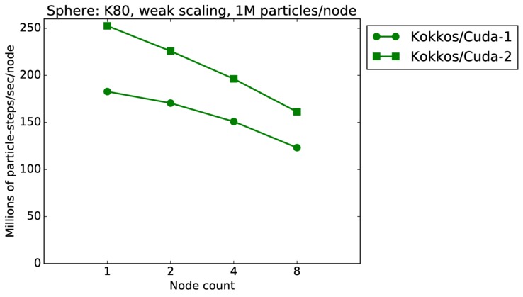
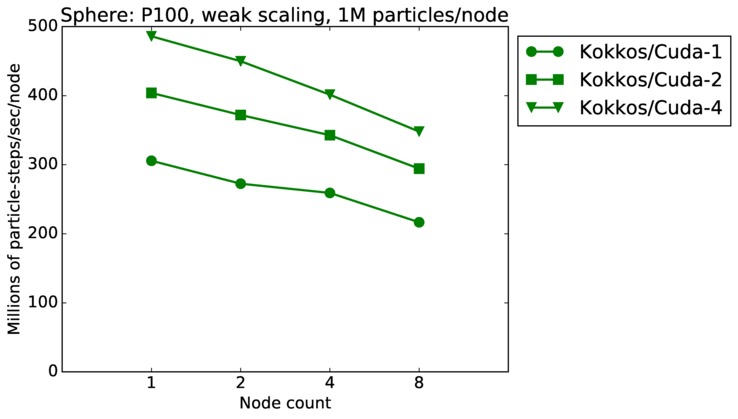
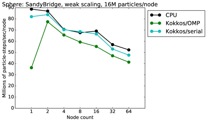
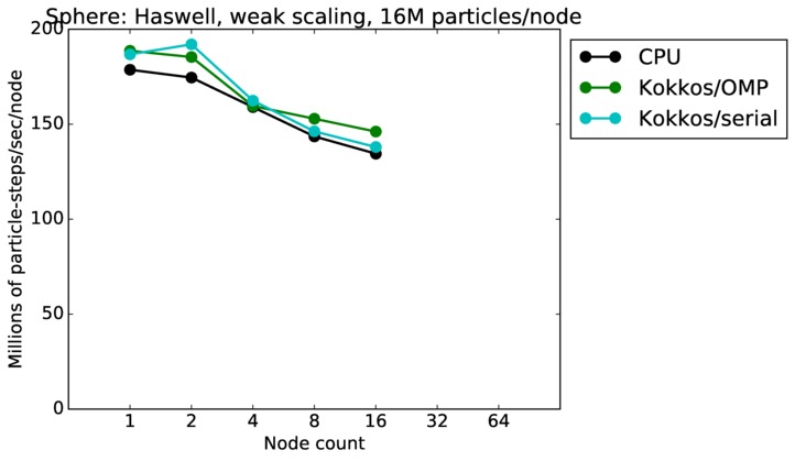
Sphere strong and weak scaling:

Fastest timing for any accelerator option running on multiple CPU or KNL or a single GPUs, as a function of node count. For strong scaling of 2 problem sizes: 8M particles, 64M particles. For weak scaling of 2 problem sizes: 1M particles/node, 16M particles/node. Only for a single GPU/node, only double precision.

Strong scaling means the same size problem is run on successively more nodes. Weak scaling means the problem size doubles each time the node count doubles. See a fuller description here of how to interpret these plots.

• Table for strong scaling of 8M particles
• Table for strong scaling of 64M particles
• Table for weak scaling of 1M particles/node
• Table for weak scaling of 16M particles/node

Sphere performance details:

• Modes: per-core, per-node, strong scaling, weak scaling
• Hardware: CPU, KNL, GPU options
• Within plot: accelerator packages, one or multiple GPUs/node

Accelerator options

SPARTA has an accelerator option implemented via the KOKKOS package, accelerator packages. The KOKKOS packages support multiple hardware options.

For acceleration on a CPU:

• CPU = reference implementation, no package, no acceleration
• Kokkos/OMP = Kokkos package with OMP option via OpenMP
• Kokkos/serial = Kokkos package with serial option for non-threaded operation on CPUs

For acceleration on an Intel KNL:

• CPU/KNL = reference implementation, no package, no acceleration
• Kokkos/KNL = Kokkos package with KNL option
• Kokkos/serial = Kokkos package with KNL/serial option

For acceleration on an NVIDIA GPU:

• Kokkos/Cuda = Kokkos package with CUDA option

Machines and node hardware

Benchmarks were run on the following machines and node hardware.

chama = Intel SandyBridge CPUs

• 1232-node cluster
• node = dual-socket Sandy Bridge:2S:8C @ 2.6 GHz, 16 cores, no hyperthreading
• interconnect = Qlogic Infiniband 4x QDR, fat tree

mutrino = Intel Haswell CPUs or Intel KNLs

• ~100 CPU nodes
• node = dual-socket Haswell 2.3 GHz CPU, 32 cores + 2x hyperthreading
• ~100 KNL nodes
• node = Knights Landing processor, 68 cores + 4x hyperthreading
• interconnect = Cray Aries Dragonfly

serrano = Intel Broadwell CPUs

• 1122-node cluster
• node = dual-socket Broadwell 2.1 GHz CPU E5-2695, 36 cores + 2x hyperthreading
• interconnect = Omni-Path

ride80 = IBM Power8 CPUs with NVIDIA K80 GPUs

• ~10 nodes
• node CPU = dual Power8 3.42 GHz CPU (Firestone), 16 cores + 8x hyperthreading
• each node has 2 Tesla K80 GPUs (each K80 is "dual" with 2 internal GPUs)
• interconnect = Infiniband

ride100 = IBM Power8 CPUs with NVIDIA P100 GPUs

• ~10 nodes
• one node = dual Power8 3.42 GHz CPU (Garrison), 16 cores + 8x hyperthreading
• each node has 2 Pascal P100 GPUs
• interconnect = Infiniband

How to build SPARTA and run the benchmarks

This table shows which accelerator packages were used on which machines:

These are the software environments on each machine and the Makefiles used to build SPARTA with different accelerator packages.

chama

• Intel 17.0.2 icc compiler, GNU 4.9.2 g++ compiler, OpenMPI-Intel 2.0
• module load intel/17.0.2.174; module load gnu/4.9.2; module load openmpi-intel/2.0
• Makefiles: Makefile.chama_cpu, Makefile.chama_kokkos_omp, Makefile.chama_kokkos_serial

mutrino

• Intel 17.0.2 icc compiler, Cray MPICH 7.5.2
• module load intel/17.0.2; module load cray-mpich/7.5.2; module load craype-haswell # for Haswell
• module load intel/17.0.2; module load cray-mpich/7.5.2; module load craype-mic-knl # for KNL
• Makefiles: Makefile.mutrino_cpu, Makefile.mutrino_kokkos_omp, Makefile.mutrino_kokkos_serial, Makefile.mutrino_knl, Makefile.mutrino_kokkos_knl, Makefile.mutrino_kokkos_serial_knl

serrano

• Intel 17.0.2 compiler, GNU 4.9.3 g++ compiler, OpenMPI-Intel 2.0
• module load intel/17.0.2.174; module load gcc/4.9.3; module load openmpi-intel/2.0
• Makefiles: Makefile.serrano_cpu, Makefile.serrano_kokkos_omp, Makefile.serrano_kokkos_serial

ride80

• GNU 4.9.3 g++ compiler, OpenMPI 1.10.5, Cuda 8.0.44
• module load openmpi/1.10.6/gcc/4.9.3/cuda/8.0.44
• Makefiles: Makefile.ride80_kokkos_cuda

ride100

• GNU 4.9.3 g++ compiler, OpenMPI 1.10.5, Cuda 8.0.44
• module load openmpi/1.10.6/gcc/4.9.3/cuda/8.0.44
• Makefiles: Makefile.ride100_kokkos_cuda

If a specific benchmark requires a build with additional package(s) installed, it is noted with the benchmark info below.

With the software environment initialized (e.g. modules loaded) and the machine Makefiles copied into src/MAKE/MINE, building SPARTA is straightforward:

cp Makefile.serrano_kokkos_omp sparta/src/MAKE/MINE   # for example
cd sparta/src
make yes-kokkos                                       # install accelerator package(s) supported by the Makefile
make serrano_kokkos_omp                               # target = suffix of Makefile.machine 

This should produce an executable named spa_machine, e.g. spa_serrano_kokkos_omp. If desired, you can copy the executable to a directory where you run the benchmark.

IMPORTANT NOTE: Achieving best performance for the benchmarks (or your own input script) on a particular machine with a particular accelerator option, requires attention to the following issues.

• mpirun command-line arguments which control how MPI tasks and threads are assigned to nodes and cores.
• SPARTA command-line arguments which invoke a specific accelerator package and its options. This may include options that are part of the package command, which can be specified in the input script, or as below, invoked from the command line.
• Some of the benchmarks use slightly-modified input scripts (indicated below), depending on which package is used. This is to boost performance of a specific accelerator option.
• Performance can be a strong function of problem size (see plots below). In addition, performance of an accelerator package can vary with MPI tasks/node, MPI tasks/GPU, threads/MPI task, or hardware threads/core (hyperthreading). In the tables below we show which choices gave best performance for specific problem sizes. But you may need to experiment for your simulation or machine.

All of the plots below include a link to a table with details on all of these issues. The table shows the mpirun (or equivalent) command used to produce each data point on each curve in the plot, the SPARTA command-line arguments used to get best performance with a particular package on that hardware, and a link to the logfile produced by the benchmark run.

How to interpret the plots

All the plots below have particles or nodes on the x-axis, and performance on the y-axis. On all the plots, better performance is up and worse performance is down. For all the plots:

• Data is normalized so that ideal performance (with respect to particle or node count) would be a horizontal line.
• If a curve trends downward (moving to the right) it means scalability is falling off. For example, in the strong-scaling plots, this is typically because the problem size/node is getting smaller as the number of nodes increases.
• If a point is missing from a curve, the simulation may have run out of memory or time, or the number of requested nodes was greater than the number of nodes on the machine.
• If a curve trends upward, scalability is increasing. For example, in the per-node plots for GPUs, simulations typically run faster (on a per-particle basis) as the system size increases.

Per-core and per-node plots:

• The y-axis is millions of particle-timesteps/sec, running on one core or an entire node.
• To infer timesteps/sec, divide the y-axis value by the number of particles in the simulation.
• The inverse of the y-axis value is sec/particle/timestep.
• To estimate how long a simulation with N particles for M timesteps will take in CPU seconds, multiply the inverse by N*M times 1 million.

Strong-scaling and weak-scaling plots:

• Strong scaling means a problem of the same size is run on successively more nodes.
• Weak scaling means the problem size is doubled each time the node count doubles. For example, if the problem size on 1 node is a million particles, then the problem size on 512 nodes is ~1/2 billion particles.
• The y-axis is millions of particle-timesteps/sec/node.
• To infer timesteps/sec, multiply the y-axis value by the number of nodes and divide by the number of particles in the simulation.
• The inverse of the y-axis value is sec-node/particle/timestep.
• To estimate how long a simulation with N particles for M timesteps on P nodes will take in CPU seconds, multiply the inverse by N*M times 1 million and divide by P.